19. One-Way ANOVA

One-way Analysis of Variance (ANOVA) is a multiple comparison technique testing whether the means of 3 or more groups are different. The hypotheses are as follows.

• \(H_0\) (null): There is no difference between the means; \(\mu_1 = \mu_2 = \ldots = \mu_n\)

• \(H_a\) (alternative): There is at least one group mean that differs from the overall mean.

ANOVA uses the F-test for testing statistical significance, which measures the ratio of the variance between groups to the variance within groups.

When there are only 2 groups, a t-test may be used instead. However, with comparing 3 or more groups, ANOVA should be used since it corrects for the family-wise error rate FWER holding the probability of a Type I error steady no matter the number of comparisons.

In this notebook, let’s see how a 1-way ANOVA relates to regression problems.

19.1. Data

Let’s generate 50 samples from 3 different normal distributions. These normal distributions are defined as follows.

• \(A \sim \mathcal{N} (0, 1)\)

• \(B \sim \mathcal{N} (1, 1)\)

• \(C \sim \mathcal{N} (1.5, 1)\)

These groups are often called treatments.

import numpy as np
import pandas as pd

np.random.seed(37)

n = 50

df = pd.concat([
    pd.DataFrame({'group': 'A', 'y': pd.Series(np.random.normal(0, 1, n))}),
    pd.DataFrame({'group': 'B', 'y': pd.Series(np.random.normal(1, 1, n))}),
    pd.DataFrame({'group': 'C', 'y': pd.Series(np.random.normal(1.5, 1, n))})
])

df.head()

	group	y
0	A	-0.054464
1	A	0.674308
2	A	0.346647
3	A	-1.300346
4	A	1.518512

19.2. Means

You can see that the empirical means and standard deviations are close to the real ones, but not exactly.

df.groupby(['group']).agg(['mean', 'std'])

	y
	mean	std
group
A	0.139065	0.998983
B	0.982454	1.057929
C	1.552792	1.052197

import matplotlib.pyplot as plt
import seaborn as sns

fig, ax = plt.subplots(1, 2, figsize=(7, 3))

sns.boxplot(df, x='group', y='y', ax=ax[0])
sns.kdeplot(df, hue='group', x='y', ax=ax[1])

fig.tight_layout()

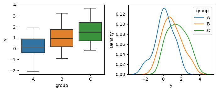
19.3. t-test

Let’s see what happens when we conduct all pairwise t-tests. You can see that group A is very different from B and C, but groups B and C are comparatively close.

from scipy import stats
from scipy import special
import itertools

def do_test(pair):
    x, y = pair

    x = df[df['group']==x]['y']
    y = df[df['group']==y]['y']

    t = stats.ttest_ind(x, y)
    s = t.statistic
    p = t.pvalue
    a = 0.05 / special.comb(3, 2) # bonferroni's correction, however, losing power

    return {
        'x': pair[0],
        'y': pair[1],
        'statistic': s,
        'pvalue': p,
        'alpha': a,
        'is_sig': p < a
    }

t_test = itertools.combinations(df['group'].unique(), 2)
t_test = map(lambda tup: do_test(tup), t_test)
t_test = pd.DataFrame(t_test)
t_test

	x	y	statistic	pvalue	alpha	is_sig
0	A	B	-4.098587	8.576614e-05	0.016667	True
1	A	C	-6.889943	5.417835e-10	0.016667	True
2	B	C	-2.702849	8.104302e-03	0.016667	True

19.4. 1-way ANOVA

Now we will apply a 1-way ANOVA. The report F statistic and p-value are shown. The test would lead us to reject the null hypothesis.

F, p = stats.f_oneway(*[df[df['group']==g]['y'] for g in ['A', 'B', 'C']])

F

23.533902104682596

p

1.3590719185638985e-09

19.5. Tukey’s HSD

Here is a post-hoc test using Tukey’s Honestly Significant Difference test. This test will see which two pair of groups are different.

hsd = stats.tukey_hsd(*[df[df['group']==g]['y'] for g in ['A', 'B', 'C']])

hsd.statistic

array([[ 0.        , -0.84338966, -1.41372695],
       [ 0.84338966,  0.        , -0.57033729],
       [ 1.41372695,  0.57033729,  0.        ]])

hsd.pvalue

array([[1.00000000e+00, 2.26787268e-04, 6.66437017e-10],
       [2.26787268e-04, 1.00000000e+00, 1.82679298e-02],
       [6.66437017e-10, 1.82679298e-02, 1.00000000e+00]])

hsd._nobs

3

hsd._ntreatments

150

hsd._stand_err

0.14661287403767

19.6. Xy, means

Before we move onto regression, keep in mind the group means and overall mean.

df.groupby(['group']).agg(['mean', 'std'])

	y
	mean	std
group
A	0.139065	0.998983
B	0.982454	1.057929
C	1.552792	1.052197

df['y'].mean()

0.8914368828670105

19.7. Regression

Here, we regress y ~ g but with g dummy-encoded (one-hot encoded).

X = df.drop(columns=['y'])
y = df['y']

from sklearn.preprocessing import OneHotEncoder

ohe = OneHotEncoder()
ohe.fit(X)

OneHotEncoder()

In a Jupyter environment, please rerun this cell to show the HTML representation or trust the notebook.
On GitHub, the HTML representation is unable to render, please try loading this page with nbviewer.org.

X = pd.DataFrame(
    ohe.transform(X).todense(),
    columns=ohe.get_feature_names_out()
)
X

	group_A	group_B	group_C
0	1.0	0.0	0.0
1	1.0	0.0	0.0
2	1.0	0.0	0.0
3	1.0	0.0	0.0
4	1.0	0.0	0.0
...	...	...	...
145	0.0	0.0	1.0
146	0.0	0.0	1.0
147	0.0	0.0	1.0
148	0.0	0.0	1.0
149	0.0	0.0	1.0

150 rows × 3 columns

from sklearn.linear_model import LinearRegression

m = LinearRegression()
m.fit(X.drop(columns=['group_A']), y)

LinearRegression()

In a Jupyter environment, please rerun this cell to show the HTML representation or trust the notebook.
On GitHub, the HTML representation is unable to render, please try loading this page with nbviewer.org.

m.intercept_, m.coef_

(0.13906468043625642, array([0.84338966, 1.41372695]))

m.coef_

array([0.84338966, 1.41372695])

19.8. Means vs coefficients

If you notice, the intercept of the regression model is the mean of A. If you add the coefficients to the intercept, you recover the means of B and C!

df.groupby(['group']).mean()

	y
group
A	0.139065
B	0.982454
C	1.552792

m.intercept_, m.coef_ + m.intercept_

(0.13906468043625642, array([0.98245434, 1.55279163]))

19.9. Test statistics vs coefficients

The coefficients are the test statistics Tukey’s HSD!

hsd.statistic

array([[ 0.        , -0.84338966, -1.41372695],
       [ 0.84338966,  0.        , -0.57033729],
       [ 1.41372695,  0.57033729,  0.        ]])

m.coef_

array([0.84338966, 1.41372695])

When using Tukey’s HSD, the p-values are given.

hsd.pvalue

array([[1.00000000e+00, 2.26787268e-04, 6.66437017e-10],
       [2.26787268e-04, 1.00000000e+00, 1.82679298e-02],
       [6.66437017e-10, 1.82679298e-02, 1.00000000e+00]])

We can also compute the p-values as below. The main complication is with computing the standard error SE.

def get_se(df):
    '''
    Computes standard error.
    Adapted from https://github.com/scipy/scipy/blob/v1.10.1/scipy/stats/_hypotests.py.
    When groups are unequal, this code should be adjusted too.
    '''
    _v = np.array([np.var(df[df['group']==g]['y'], ddof=1) for g in df['group'].unique()])
    _s = np.array([df[df['group']==g].shape[0] - 1 for g in df['group'].unique()])
    _n = df.shape[0] - df['group'].unique().shape[0]
    _mse = np.sum(_v * _s) / _n
    _norm = 2 / df[df['group']=='A'].shape[0]
    _se = np.sqrt(_norm * _mse / 2)

    return _se

def get_pvalue(m_0, m_1, se, k, dof):
    diff = np.abs(m_0 - m_1)
    t = diff / se
    print(f'{t=}, {k=}, {dof=}')
    return stats.distributions.studentized_range.sf(t, k, dof)

_mean = df.groupby(['group']).mean()['y'].to_numpy()
_se = get_se(df)
_k = df['group'].unique().shape[0]
_dof = df.shape[0] - _k

_mean

array([0.13906468, 0.98245434, 1.55279163])

_se

0.14661287403767

_k

3

_dof

147

get_pvalue(_mean[0], _mean[1], _se, _k, _dof)

t=5.752493850354061, k=3, dof=147

0.00022678726812552785

get_pvalue(_mean[0], _mean[2], _se, _k, _dof)

t=9.64258398375435, k=3, dof=147

6.664370166831191e-10

get_pvalue(_mean[1], _mean[2], _se, _k, _dof)

t=3.8900901334002893, k=3, dof=147

0.01826792981617653

Here’s yet another way to compute the p-values.

1 - stats.studentized_range.cdf(np.abs(_mean[0] - _mean[1]) / _se, _k, _dof)

0.00022678726812552785

1 - stats.studentized_range.cdf(np.abs(_mean[0] - _mean[2]) / _se, _k, _dof)

6.664370166831191e-10

1 - stats.studentized_range.cdf(np.abs(_mean[1] - _mean[2]) / _se, _k, _dof)

0.01826792981617653