3. Optimizing Marginal Revenue from the Demand Curve
The demand curve is usually defined as a plot of demand/quantity (y-axis), \(Q\), against the price (x-axis), \(P\). For nearly all products, as \(P\) goes up then \(Q\) comes down. We can model the demand curve (linearly or non-linearly) to figure out how \(P\) and \(Q\) are related, and use this relationship to find the “optimal” price that will maximize marginal revenue. Let’s see how computing the optimal price from a demand curve works.
3.1. Simulated data
Let’s simulate some data for \(P\) and \(Q\).
\(P \sim \mathcal{N}(40, 20)\)
\(Q \sim \mathcal{N}(400 - 5.0 P, 1)\)
[1]:
import pandas as pd
import numpy as np

np.random.seed(37)

N = 100
P = np.random.normal(40, 20, N) # np.arange(0, 81, 1)
Q = np.random.normal(400 + (-5 * P), 1, P.shape[0]) + np.random.normal(10, 20, N)

df = pd.DataFrame({'p': P, 'q': Q}) \
    .sort_values(['p']) \
    .query('p >= 0') \
    .reset_index(drop=True)

df.shape
[1]:
(97, 2)
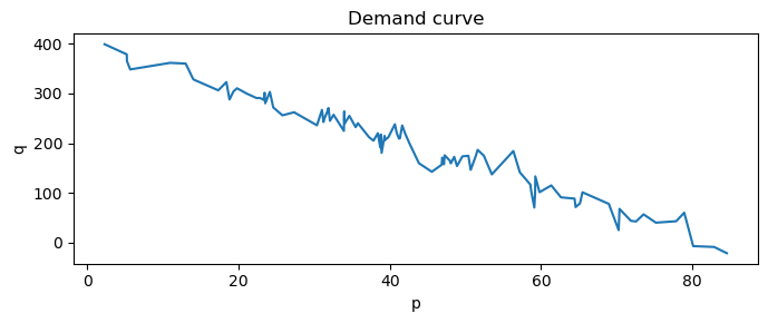
As you can see below, the demand curve is not smooth and often times, this seesaw curve is the empirical demand curve of a lot of products. We need to smooth it out.
[2]:
import matplotlib.pyplot as plt

f, a = plt.subplots(figsize=(7, 3))

df.set_index(['p'])['q'] \
    .plot(
        kind='line',
        ax=a,
        title='Demand curve',
        ylabel='q'
    )

f.tight_layout()
3.2. Modeling
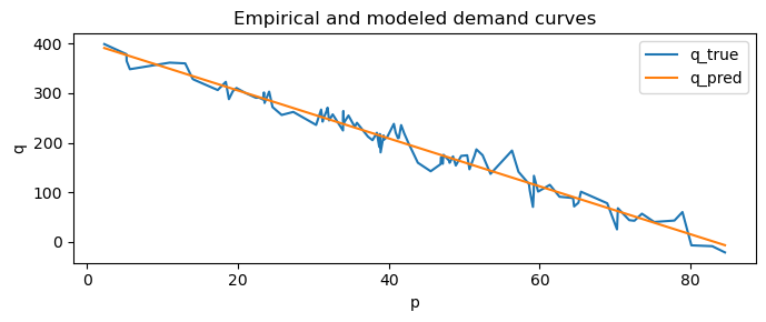
We can model the demand curve with linear regression. The linear regression model of the demand curve is a straight line (it smooths out the empirical demand curve).
\(Q \sim P\)
[3]:
from sklearn.linear_model import LinearRegression

X = df[['p']]
y = df['q']

qp_model = LinearRegression()
qp_model.fit(X, y)

qp_model.intercept_, qp_model.coef_
[3]:
(402.0611487648074, array([-4.83565712]))
[4]:
pred_df = df.assign(q_pred=qp_model.predict(X))

f, a = plt.subplots(figsize=(7, 3))

pred_df \
    .rename(columns={'q': 'q_true'}) \
    .set_index(['p']) \
    .plot(
        kind='line',
        ax=a,
        title='Empirical and modeled demand curves',
        ylabel='q'
    )

f.tight_layout()
3.3. Marginal revenue optimization
From the linear regression model of the demand curve, we have the following relationships from the model.
\(Q = 401.96 - 4.8 P\)
\(P = 83.74 - 0.21 Q\)
We know the following about total revenue, \(R\).
\(R = P Q\)
\(R = \left(83.74 - 0.21 Q \right) Q\)
\(R = 83.74Q - 0.21 Q^2\)
The marginal revenue is \(R' = \dfrac{\mathrm{d} R}{\mathrm{d} Q}\).
\(R' = \dfrac{\mathrm{d} R}{\mathrm{d} Q} = 83.74 - 0.42 Q\)
The marginal cost, \(C'\), of producing a unit is (given as) 15.0. The optimal price can be found when we set \(R' = C'\) and solve for \(Q\) and plug back in \(Q\) to get \(P\).
\(R' = C'\)
\(83.74 - 0.42 Q = 15.0\)
\(-0.42 Q = -68.74\)
\(Q = 163.67\)
Since we know \(P = 83.74 - 0.21 Q\), we plug \(Q\) in to get the price.
\(P = 83.74 - 0.21 Q\)
\(P = 83.74 - 0.21 (163.67)\)
\(P = 49.37\)
Let’s compute \(R = PQ\).
\(R = PQ\)
\(R = 49.37 \times 163.67\)
\(R = 8,080.39\)
Let’s compute \(R'\).
\(R' = 83.74 - 0.42 Q\)
\(R' = 83.74 - 0.42 (163.67)\)
\(R' = 15.00\)
Let’s define the profit, \(T\), as follows, and plug in the values.
\(T = PQ - C'Q\)
\(T = (49.37 \times 163.67) - (15 \times 163.67)\)
\(T = 5,625.34\)
[5]:
def get_pq(b_0, b_1):
    return lambda q: (-b_0 / b_1) + (1 / b_1) * q

def get_qp(b_0, b_1):
    return lambda p: b_0 + (b_1 * p)

def get_mr(b_0, b_1):
    return lambda q: (-b_0 / b_1) + (2 * (1 / b_1) * q)

def get_qo(b_0, b_1):
    z_0 = (-b_0 / b_1)
    z_1 = 2 * (1 / b_1)
    return lambda mc: (mc - z_0) / z_1

def get_funcs(b_0, b_1):
    pq = get_pq(b_0, b_1)
    qp = get_qp(b_0, b_1)
    mr = get_mr(b_0, b_1)
    qo = get_qo(b_0, b_1)
    r = lambda p, q: p * q
    t = lambda p, q, mc: (p * q) - (mc * q)

    return pq, qp, mr, qo, r, t

def get_opt(f, mc):
    pq_f, qp_f, mr_f, qo_f, r_f, t_f = f

    q_opt = qo_f(mc)
    p_opt = pq_f(q_opt)
    mr_opt = mr_f(q_opt)
    r_opt = r_f(p_opt, q_opt)
    t_opt = t_f(p_opt, q_opt, mc)

    return pd.Series({
        'mc': mc,
        'q_opt': q_opt,
        'p_opt': p_opt,
        'mr_opt': mr_opt,
        'r_opt': r_opt,
        't_opt': t_opt
    })

f = get_funcs(qp_model.intercept_, qp_model.coef_[0])
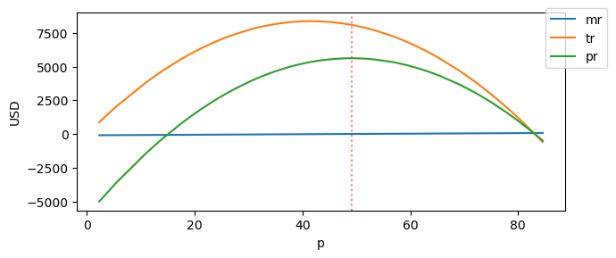
For this product, the optimal price is 49.08 which will lead to
164.72 units sold (quantity),
8,084.68 USD in revenue, and
5,613,77 USD in profit.
[6]:
get_opt(f, 15)
[6]:
mc          15.000000
q_opt      164.763146
p_opt       49.072545
mr_opt      15.000000
r_opt     8085.346941
t_opt     5613.899751
dtype: float64
The plot below shows the marginal revenue mr, total revenue tr and profit pr at each price point p. The vertical red dotted line marks the optimal price and it intersects with the profit curve an its highest point.
[7]:
fig, ax = plt.subplots(figsize=(7, 3))

pred_df \
    .assign(
        mr=lambda d: f[2](d['q_pred']),
        tr=lambda d: f[4](d['p'], d['q_pred']),
        pr=lambda d: f[5](d['p'], d['q_pred'], 15)
    ) \
    .set_index(['p'])[['mr', 'tr', 'pr']] \
    .plot(kind='line', ylabel='USD', ax=ax)

ax.axvline(x=get_opt(f, 15).p_opt, color='r', alpha=0.5, linestyle='dotted')
ax.legend(bbox_to_anchor=(1.1, 1.05))

fig.tight_layout()