20. Optimizing a Function

In this notebook, we will explore how to find the optimal parameters of some function.

20.1. Data

Let’s simulate data.

\(z = f(x, y) = \sin \left( \sqrt{x^2 + y^2} \right)\)

import pandas as pd
import numpy as np

x = np.arange(-5, 5, 0.25)
y = np.arange(-5, 5, 0.25)
x, y = np.meshgrid(x, y)
z = np.sin(np.sqrt(x**2 + y**2))

df = pd.DataFrame([(_x, _y, _z) for _x, _y, _z in zip(np.ravel(x), np.ravel(y), np.ravel(z))],
                  columns=['x', 'y', 'z'])

x.shape, y.shape, z.shape, df.shape

((40, 40), (40, 40), (40, 40), (1600, 3))

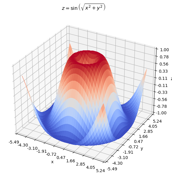
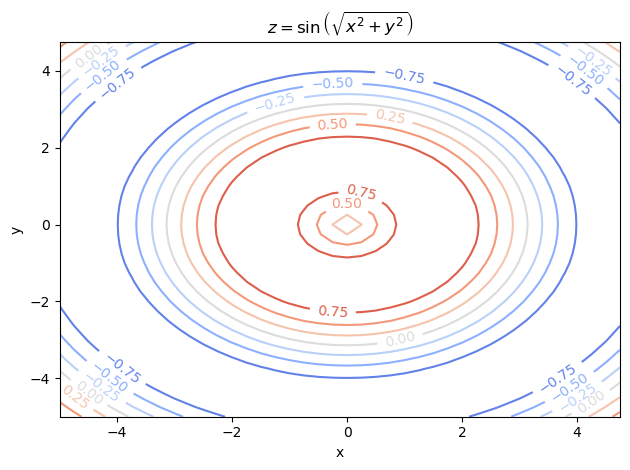
20.2. Surface plot, Matplotlib

As you can see from the surface and contour plots below, the optimal parameters \(\theta = (x, y)\) should produce \(z \sim 1\) and is near the center of the graph (but not actually the center).

import matplotlib.pyplot as plt
from matplotlib import cm
from matplotlib.ticker import LinearLocator
import numpy as np

fig, ax = plt.subplots(
    subplot_kw={'projection': '3d'},
    figsize=(6, 6)
)

surf = ax.plot_surface(x, y, z, cmap=cm.coolwarm, linewidth=0, antialiased=False)

ax.set_xlabel('x')
ax.set_ylabel('y')
ax.set_zlabel('z')
ax.xaxis.set_major_locator(LinearLocator(10))
ax.yaxis.set_major_locator(LinearLocator(10))
ax.zaxis.set_major_locator(LinearLocator(10))
ax.xaxis.set_major_formatter('{x:.02f}')
ax.yaxis.set_major_formatter('{x:.02f}')
ax.zaxis.set_major_formatter('{x:.02f}')
ax.set_title(r'$z = \sin \left( \sqrt{x^2 + y^2} \right)$')

fig.tight_layout()

fig, ax = plt.subplots()

qcs = ax.contour(x, y, z, cmap=cm.coolwarm)
ax.clabel(qcs, inline=1, fontsize=10)
ax.set_title(r'$z = \sin \left( \sqrt{x^2 + y^2} \right)$')
ax.set_xlabel('x')
ax.set_ylabel('y')

fig.tight_layout()

20.3. Surface plot, Plotly

The static Matplotlib surface plot makes it hard to inspect the graph. A surface plot using Plotly is better since you can rotate the graph and inspect it.

import plotly.graph_objects as go

fig = go.Figure(data=[go.Surface(
    x=x,
    y=y,
    z=z,
    colorscale='Viridis',
    opacity=0.5,
)])

fig.update_layout(
    title=r'$z = \sin \left( \sqrt{x^2 + y^2} \right)$',
    autosize=False,
    width=600,
    height=600,
    margin={'l': 65, 'r': 50, 'b': 65, 't': 90}
)
fig.update_xaxes(title='x')
fig.update_yaxes(title='y')

fig.show()

fig = go.Figure(data =
    go.Contour(
        z=z,
        x=df['x'].unique(),
        y=df['y'].unique(),
        colorscale='Viridis'
    ))
fig.update_layout(
    title=r'$z = \sin \left( \sqrt{x^2 + y^2} \right)$',
    autosize=False,
    width=600,
    height=600,
    margin={'l': 65, 'r': 50, 'b': 65, 't': 90}
)

fig.show()

20.4. Optimal points

Since we simulated the data, we obviously know which points produces the optimal \(z\) values. There are several of them.

df[df['z']==df['z'].max()]

	x	y	z
578	-0.5	-1.5	0.999947
582	0.5	-1.5	0.999947
734	-1.5	-0.5	0.999947
746	1.5	-0.5	0.999947
894	-1.5	0.5	0.999947
906	1.5	0.5	0.999947
1058	-0.5	1.5	0.999947
1062	0.5	1.5	0.999947

20.5. Modeling

We can use a random forest model to approximate the function.

from sklearn.ensemble import RandomForestRegressor

m = RandomForestRegressor(random_state=37, n_jobs=-1, n_estimators=50)
m.fit(df[['x', 'y']], df['z'])

RandomForestRegressor(n_estimators=50, n_jobs=-1, random_state=37)

The non-validated error is pretty good.

from sklearn.metrics import mean_absolute_error

mean_absolute_error(df['z'], m.predict(df[['x', 'y']]))

0.011997664199503578

If we visulize the surface plot using the predicted \(\hat{z}\), you can see we have done a great job recovering the original surface plot.

_x, _y = np.meshgrid(np.arange(-5, 5, 0.25), np.arange(-5, 5, 0.25))
_z = m.predict(pd.DataFrame([(_x_val, _y_val) for _x_val, _y_val in zip(np.ravel(_x), np.ravel(_y))], columns=['x', 'y'])).reshape(_x.shape)

_x.shape, _y.shape, _z.shape

((40, 40), (40, 40), (40, 40))

fig = go.Figure(data=[go.Surface(
    x=_x,
    y=_y,
    z=_z,
    colorscale='Viridis',
    opacity=0.5,
)])

fig.update_layout(
    title=r'$\hat{z} = \sin \left( \sqrt{x^2 + y^2} \right)$',
    autosize=False,
    width=600,
    height=600,
    margin={'l': 65, 'r': 50, 'b': 65, 't': 90}
)
fig.update_xaxes(title='x')
fig.update_yaxes(title='y')

fig.show()

20.6. Optimizing, Optuna

To find the optimal parameters, we can use Optuna to search for the best parameters.

import optuna

optuna.logging.set_verbosity(optuna.logging.WARNING)

def objective(trial, m):
    x = trial.suggest_float('x', -4, 4)
    y = trial.suggest_float('y', -4, 4)
    _df = pd.DataFrame([[x, y]], columns=['x', 'y'])
    z = m.predict(_df)

    return z[0]

study = optuna.create_study(**{
    'study_name': 'opt-study',
    'storage': 'sqlite:///_temp/opt-study.db',
    'load_if_exists': True,
    'direction': 'maximize',
    'sampler': optuna.samplers.TPESampler(seed=37),
    'pruner': optuna.pruners.MedianPruner(n_warmup_steps=10)
})

study.optimize(**{
    'func': lambda t: objective(t, m),
    'n_trials': 200,
    'n_jobs': 6,
    'show_progress_bar': True
})

/opt/anaconda3/lib/python3.9/site-packages/optuna/progress_bar.py:49: ExperimentalWarning:

Progress bar is experimental (supported from v1.2.0). The interface can change in the future.

Optuna does a decent job of finding the near-optimal parameters.

study.best_params

{'x': 1.555609216974581, 'y': -0.2773733254268651}

study.best_value

0.9971038658796584

20.7. Optimizing, Scipy

We can also find the optimal parameters using Scipy.

import scipy.optimize as optimize

def f(tup):
    x, y = tup
    z = np.sin(np.sqrt(x ** 2 + y ** 2))
    return -z

p_opt = optimize.fmin(f, np.array([0, 0]), ftol=1e-30, xtol=1e-30, maxiter=10_000, maxfun=10_000)
p_opt

Optimization terminated successfully.
         Current function value: -1.000000
         Iterations: 97
         Function evaluations: 266

array([1.54456722, 0.28585516])

The parameters found from Scipy is even more optimal than the ones we get from the data or Optuna!

pd.Series([
    -f(p_opt),
    -f(np.array([0.5, 1.5])),
    -f(np.array([study.best_params['x'], study.best_params['y']]))
], ['scipy', 'data', 'optuna'])

scipy     1.000000
data      0.999947
optuna    0.999956
dtype: float64