4. Poisson Regression, Gradient Descent

In this notebook, we will show how to use gradient descent to solve a Poisson regression model. A Poisson regression model takes on the following form.

\(\operatorname{E}(Y\mid\mathbf{x})=e^{\boldsymbol{\theta}' \mathbf{x}}\)

where

• \(x\) is a vector of input values

• \(\theta\) is a vector weights (the coefficients)

• \(y\) is the expected value of the parameter for a Poisson distribution, typically, denoted as \(\lambda\)

Note that Scikit-Learn does not provide a solver a Poisson regression model, but statsmodels does, though examples for the latter is thin.

4.1. Simulate data

Now, let’s simulate the data. Note that the coefficients are \([1, 0.5, 0.2]\) and that there is error \(\epsilon \sim \mathcal{N}(0, 1)\) added to the simulated data.

\(y=e^{1 + 0.5x_1 + 0.2x_2 + \epsilon}\)

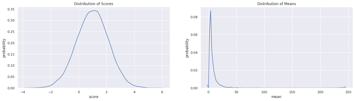
In this notebook, the score is denoted as \(z\) and \(z = 1 + 0.5x_1 + 0.2x_2 + \epsilon\). Additionally, \(y\) is the mean for a Poisson distribution. The variables \(X_1\) and \(X_2\) are independently sampled from their own normal distribution \(\mathcal{N}(0, 1)\).

After we simulate the data, we will plot the distribution of the scores and means. Note that the expected value of the output \(y\) is 5.2.

%matplotlib inline
import numpy as np
import matplotlib.pyplot as plt
import seaborn as sns
from numpy.random import normal
from scipy.stats import poisson

np.random.seed(37)
sns.set(color_codes=True)

n = 10000
X = np.hstack([
    np.array([1 for _ in range(n)]).reshape(n, 1),
    normal(0.0, 1.0, n).reshape(n, 1),
    normal(0.0, 1.0, n).reshape(n, 1)
])
z = np.dot(X, np.array([1.0, 0.5, 0.2])) + normal(0.0, 1.0, n)
y = np.exp(z)

4.2. Visualize data

fig, ax = plt.subplots(1, 2, figsize=(20, 5))

sns.kdeplot(z, ax=ax[0])
ax[0].set_title(r'Distribution of Scores')
ax[0].set_xlabel('score')
ax[0].set_ylabel('probability')

sns.kdeplot(y, ax=ax[1])
ax[1].set_title(r'Distribution of Means')
ax[1].set_xlabel('mean')
ax[1].set_ylabel('probability')

Text(0, 0.5, 'probability')

4.3. Solve for the Poisson regression model weights

Now we learn the weights of the Poisson regression model using gradient descent. Notice that the loss function of a Poisson regression model is identical to an Ordinary Least Square (OLS) regression model?

\(L(\theta) = \frac{1}{n} (\hat{y} - y)^2\)

We do not have to worry about writing out the gradient of the loss function since we are using Autograd.

import autograd.numpy as np
from autograd import grad
from autograd.numpy import exp, log, sqrt

# define the loss function
def loss(w, X, y):
    y_pred = np.exp(np.dot(X, w))
    loss = ((y_pred - y) ** 2.0)
    return loss.mean(axis=None)

#the magic line that gives you the gradient of the loss function
loss_grad = grad(loss)

def learn_weights(X, y, alpha=0.05, max_iter=30000, debug=False):
    w = np.array([0.0 for _ in range(X.shape[1])])

    if debug is True:
        print('initial weights = {}'.format(w))

    loss_trace = []
    weight_trace = []

    for i in range(max_iter):
        loss = loss_grad(w, X, y)
        w = w - (loss * alpha)
        if i % 2000 == 0 and debug is True:
            print('{}: loss = {}, weights = {}'.format(i, loss, w))

        loss_trace.append(loss)
        weight_trace.append(w)

    if debug is True:
        print('intercept + weights: {}'.format(w))

    loss_trace = np.array(loss_trace)
    weight_trace = np.array(weight_trace)

    return w, loss_trace, weight_trace

def plot_traces(w, loss_trace, weight_trace, alpha):
    fig, ax = plt.subplots(1, 2, figsize=(20, 5))

    ax[0].set_title(r'Log-loss of the weights over iterations, $\alpha=${}'.format(alpha))
    ax[0].set_xlabel('iteration')
    ax[0].set_ylabel('log-loss')
    ax[0].plot(loss_trace[:, 0], label=r'$\beta$')
    ax[0].plot(loss_trace[:, 1], label=r'$x_0$')
    ax[0].plot(loss_trace[:, 2], label=r'$x_1$')
    ax[0].legend()

    ax[1].set_title(r'Weight learning over iterations, $\alpha=${}'.format(alpha))
    ax[1].set_xlabel('iteration')
    ax[1].set_ylabel('weight')
    ax[1].plot(weight_trace[:, 0], label=r'$\beta={:.2f}$'.format(w[0]))
    ax[1].plot(weight_trace[:, 1], label=r'$x_0={:.2f}$'.format(w[1]))
    ax[1].plot(weight_trace[:, 2], label=r'$x_1={:.2f}$'.format(w[2]))
    ax[1].legend()

We try learning the coefficients with different learning weights \(\alpha\). Note the behavior of the traces of the loss and weights for different \(\alpha\)? The loss function was the same one used for OLS regression, but the loss function for Poisson regression is defined differently. Nevertheless, we still get acceptable results.

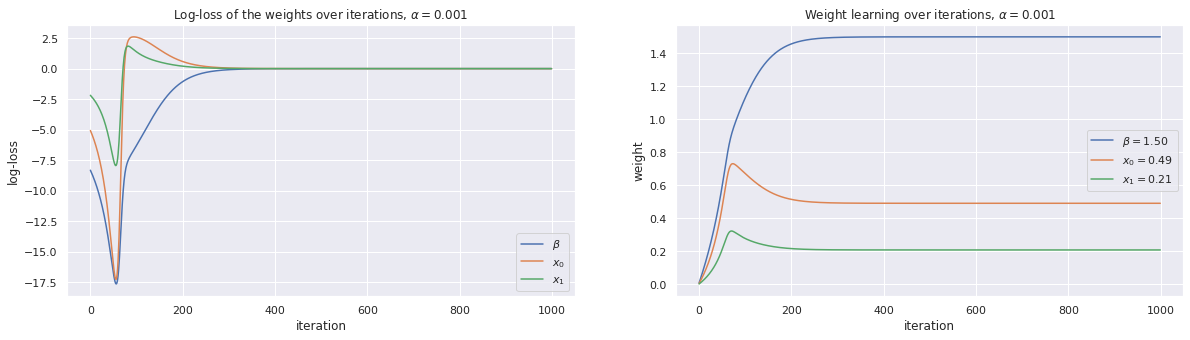
4.3.1. Use gradient descent with \(\alpha=0.001\)

alpha = 0.001
w, loss_trace, weight_trace = learn_weights(X, y, alpha=alpha, max_iter=1000)
plot_traces(w, loss_trace, weight_trace, alpha=alpha)
print(w)

[1.50066529 0.49134304 0.20836951]

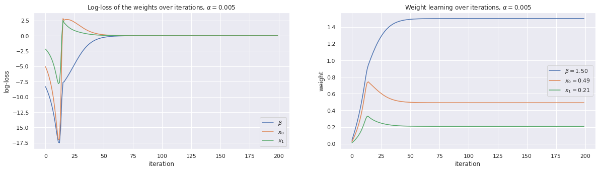
4.3.2. Use gradient descent with \(\alpha=0.005\)

alpha = 0.005
w, loss_trace, weight_trace = learn_weights(X, y, alpha=alpha, max_iter=200)
plot_traces(w, loss_trace, weight_trace, alpha=alpha)
print(w)

[1.50066529 0.49134304 0.20836951]

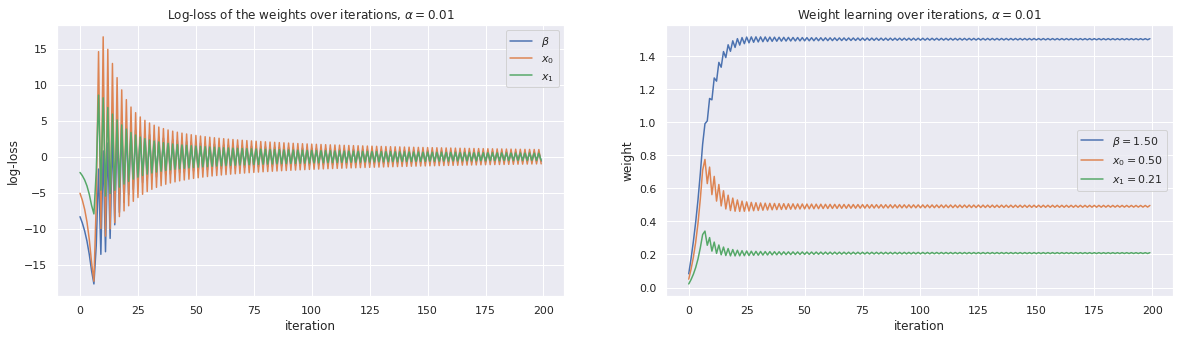
4.3.3. Use gradient descent with \(\alpha=0.01\)

alpha = 0.01
w, loss_trace, weight_trace = learn_weights(X, y, alpha=alpha, max_iter=200)
plot_traces(w, loss_trace, weight_trace, alpha=alpha)
print(w)

[1.50393889 0.49616052 0.21077159]