14. Explanation vs Prediction
In this notebook, we start with the philosophical argument that explanatory modeling is a fundamentally different exercise with a different goal from predictive modeling. Explanatory models are meant to discover the narratives of outcomes (looking backwards to the past) while predictive models are meant to best guess outcomes (looking forwards to the future). We might as well add that causal modeling is different from both as well, as causal models are meant to discover how to change
outcomes.
Typically, for a probabilistic classifier, the Area Under the Curve (AUC) for the Receiver Operating Characteristic (ROC) and Precision-Recall (PR) curves are used to judge the performance of such a classifier. AUC-ROC is more dominant in the certain fields, but AUC-PR is more appropriate when there is class imbalance with the data. These performance measures are entirely appropriate when used in predictive modeling as you want to see if a model can generalize into the future on unseen data.
Sometimes, probabilistic classifiers are learned for explanatory purpose, and prediction is a secondary concern, if at all. Common approaches to building models for explanatory purpose often involves stepwise, greedy search for features to add that will improve the model. A usual performance measure to test if a feature/variable should be added includes computing the likelihood of the model (eg. \(P(D|M)\) where \(D\) is the data and \(M\) is the model). Computing the likelihood of a model may be intractable, however. Another way to judge a model is to use something like r-squared. At heart, r-squared compares the lift of the alternative model with a reference (or null) model. Although not identical to r-squared, a host of pseudo r-squared have been invented for logistic regression. We can reason that if we find an r-squared like measure to judge a probabilistic classifier, we can use such measure the explanatory performance of the model.
Proper scoring rules like the Brier Score (BS) are wholly appropriate to judge probabilistic classifiers (even more than quasi-proper and improper scoring rules). It is said that the BS is to the Brier Skill Score (BSS) as Mean Squared Error (MSE) is to r-squared. We argue that you can use the BSS for model selection in choosing among different explanatory models. We show how to do so in this notebook, including how choosing an optimal explantory model may mean choosing a sub-optimal predictive model (and vice-versa).
14.1. Load data
Let’s import a dataset about students and whether they have conducted research. The indepent variables in X are the student’s scores and peformance measures, and the dependent variable y is whether they have done research (y = 1) or not (y = 0).
[1]:
import pandas as pd
import numpy as np

url = 'https://raw.githubusercontent.com/selva86/datasets/master/Admission.csv'
Xy = pd.read_csv(url) \
    .drop(columns=['Chance of Admit ', 'Serial No.'])

X = Xy.drop(columns=['Research'])
y = Xy['Research']

X.shape, y.shape
[1]:
((400, 6), (400,))
14.2. Split data
Here, we split the data into 10% testing and 90% training while preserving the proportion of y in both folds.
[87]:
from sklearn.model_selection import StratifiedKFold

tr_idx, te_idx = next(StratifiedKFold(n_splits=10, random_state=37, shuffle=True).split(X, y))

X_tr, X_te = X.iloc[tr_idx], X.iloc[te_idx]
y_tr, y_te = y.iloc[tr_idx], y.iloc[te_idx]

X_tr.shape, y_tr.shape, X_te.shape, y_te.shape
[87]:
((360, 6), (360,), (40, 6), (40,))
[88]:
y_tr.value_counts() / y_tr.value_counts().sum()
[88]:
Research
1    0.547222
0    0.452778
Name: count, dtype: float64
[89]:
y_te.value_counts() / y_te.value_counts().sum()
[89]:
Research
1    0.55
0    0.45
Name: count, dtype: float64
14.3. Model
To start off, we will model the data using a logistic regression model. All the features will be used, and so we will call this model a saturated one.
[5]:
from sklearn.linear_model import LogisticRegression

m = LogisticRegression(n_jobs=-1, random_state=37, solver='saga', max_iter=10_000)
m.fit(X_tr, y_tr)
[5]:
LogisticRegression(max_iter=10000, n_jobs=-1, random_state=37, solver='saga')In a Jupyter environment, please rerun this cell to show the HTML representation or trust the notebook.
On GitHub, the HTML representation is unable to render, please try loading this page with nbviewer.org.
LogisticRegression(max_iter=10000, n_jobs=-1, random_state=37, solver='saga')
14.4. Score
Now let’s look at some scores for the null and saturated models.
roc: AUC-ROC
aps: AUC-PR
brier: BS
log: log loss
14.4.1. Null model
Clearly below, you can see that the null model has no predictive power since AUC-ROC is no better than chance (50%) and AUC-PR is also no better than chance (the average percision score is equal to the climatic average). With the BS and log loss score, lower is better, but we have no idea if these are good are bad since we have no other model to compare with, yet.
[90]:
from sklearn.metrics import roc_auc_score, average_precision_score, brier_score_loss, log_loss

p1 = (y_tr.value_counts() / y_tr.value_counts().sum()).sort_index().loc[1]
y_pred = np.full(y_te.shape, p1)

pd.Series([
    roc_auc_score(y_te, y_pred),
    average_precision_score(y_te, y_pred),
    brier_score_loss(y_te, y_pred),
    log_loss(y_te, y_pred)
], ['roc', 'aps', 'brier', 'log'])
[90]:
roc      0.500000
aps      0.550000
brier    0.247508
log      0.688154
dtype: float64
14.4.2. Saturated model
The saturated model is definitely doing better than chance at predicting as indicated by AUC-ROC and AUC-PR. We see that both BS and log loss score are also lower, and so the saturateed model better explains the the variance we see in the data.
[14]:
y_pred = m.predict_proba(X_te)[:,1]

pd.Series([
    roc_auc_score(y_te, y_pred),
    average_precision_score(y_te, y_pred),
    brier_score_loss(y_te, y_pred),
    log_loss(y_te, y_pred)
], ['roc', 'aps', 'brier', 'log'])
[14]:
roc      0.768246
aps      0.747516
brier    0.194466
log      0.580401
dtype: float64
14.5. Model search
Here, we do a model search. Since there are 6 independent variables, there are \(C^6_6 + C^6_5 + C^6_4 + C^6_3 + C^6_2 + C^6_1 = 63\) possible combinations of variables.
[86]:
import itertools

models = itertools.chain(*[itertools.combinations(X.columns, i) for i in range(1, X.shape[1] + 1)])
models = map(lambda x: list(x), models)
models = list(models)

len(models)
[86]:
63
For each possible combination of variables, we learn a logistic regression model and compute performance measures.
roc: AUC-ROC
aps: AUC-PR
brier_null: BS for the null model
brier_pred: BS for the model (of the specified combination of features)
bss: BSS for the model
log_null: log loss score for the null model
log_pred: log loss score for the model
lss: log loss skill score for the model
[80]:
def get_performance(columns, X_tr, y_tr, X_te, y_te):
    m = LogisticRegression(n_jobs=-1, random_state=37, solver='saga', max_iter=10_000)
    m.fit(X_tr[columns], y_tr)

    p1 = (y_tr.value_counts() / y_tr.value_counts().sum()).sort_index().loc[1]
    y_null = np.full(y_te.shape, p1)
    y_pred = m.predict_proba(X_te[columns])[:,1]

    b_null = brier_score_loss(y_te, y_null)
    b_pred = brier_score_loss(y_te, y_pred)
    bss = 1 - (b_pred / b_null)

    l_null = log_loss(y_te, y_null)
    l_pred = log_loss(y_te, y_pred)
    lss = 1 - (l_pred / l_null)

    p = pd.Series([
        roc_auc_score(y_te, y_pred),
        average_precision_score(y_te, y_pred),
        b_null,
        b_pred,
        bss,
        l_null,
        l_pred,
        lss
    ], ['roc', 'aps', 'brier_null', 'brier_pred', 'bss', 'log_null', 'log_pred', 'lss'])

    return p

r = pd.DataFrame({'|'.join(m): get_performance(m, X_tr, y_tr, X_te, y_te) for m in models}).T
r
[80]:
| roc | aps | brier_null | brier_pred | bss | log_null | log_pred | lss | |
|---|---|---|---|---|---|---|---|---|
| GRE Score | 0.851224 | 0.870199 | 0.248012 | 0.247035 | 0.003937 | 0.689166 | 0.687184 | 0.002876 |
| TOEFL Score | 0.803616 | 0.830837 | 0.248012 | 0.229693 | 0.073862 | 0.689166 | 0.651750 | 0.054292 |
| University Rating | 0.761285 | 0.752031 | 0.248012 | 0.195166 | 0.213080 | 0.689166 | 0.580746 | 0.157320 |
| SOP | 0.762183 | 0.735531 | 0.248012 | 0.194738 | 0.214804 | 0.689166 | 0.581555 | 0.156146 |
| LOR | 0.735010 | 0.733848 | 0.248012 | 0.207188 | 0.164606 | 0.689166 | 0.602331 | 0.126000 |
| ... | ... | ... | ... | ... | ... | ... | ... | ... |
| GRE Score|TOEFL Score|University Rating|LOR |CGPA | 0.762632 | 0.768483 | 0.248012 | 0.198189 | 0.200889 | 0.689166 | 0.585421 | 0.150537 |
| GRE Score|TOEFL Score|SOP|LOR |CGPA | 0.761060 | 0.737548 | 0.248012 | 0.199990 | 0.193625 | 0.689166 | 0.590588 | 0.143039 |
| GRE Score|University Rating|SOP|LOR |CGPA | 0.773411 | 0.754668 | 0.248012 | 0.192660 | 0.223183 | 0.689166 | 0.576357 | 0.163689 |
| TOEFL Score|University Rating|SOP|LOR |CGPA | 0.770716 | 0.750870 | 0.248012 | 0.193978 | 0.217868 | 0.689166 | 0.581121 | 0.156776 |
| GRE Score|TOEFL Score|University Rating|SOP|LOR |CGPA | 0.768246 | 0.747516 | 0.248012 | 0.194466 | 0.215902 | 0.689166 | 0.580401 | 0.157821 |
63 rows × 8 columns
14.5.1. Best models, ROC
The best model based on AUC-ROC is the one with a single variable, GRE Score.
[81]:
r.sort_values(['roc'], ascending=False).head(5)
[81]:
| roc | aps | brier_null | brier_pred | bss | log_null | log_pred | lss | |
|---|---|---|---|---|---|---|---|---|
| GRE Score | 0.851224 | 0.870199 | 0.248012 | 0.247035 | 0.003937 | 0.689166 | 0.687184 | 0.002876 |
| SOP|CGPA | 0.831574 | 0.854039 | 0.248012 | 0.169722 | 0.315671 | 0.689166 | 0.517150 | 0.249601 |
| CGPA | 0.831125 | 0.857370 | 0.248012 | 0.170853 | 0.311110 | 0.689166 | 0.523775 | 0.239987 |
| SOP|LOR |CGPA | 0.830227 | 0.857736 | 0.248012 | 0.171121 | 0.310029 | 0.689166 | 0.519056 | 0.246834 |
| University Rating|CGPA | 0.828543 | 0.852778 | 0.248012 | 0.170621 | 0.312046 | 0.689166 | 0.523330 | 0.240633 |
14.5.2. Best models, APS
The best model based on AUC-PR is also the one with only GRE Score.
[82]:
r.sort_values(['aps'], ascending=False).head(5)
[82]:
| roc | aps | brier_null | brier_pred | bss | log_null | log_pred | lss | |
|---|---|---|---|---|---|---|---|---|
| GRE Score | 0.851224 | 0.870199 | 0.248012 | 0.247035 | 0.003937 | 0.689166 | 0.687184 | 0.002876 |
| LOR |CGPA | 0.825960 | 0.858192 | 0.248012 | 0.172072 | 0.306196 | 0.689166 | 0.522815 | 0.241380 |
| SOP|LOR |CGPA | 0.830227 | 0.857736 | 0.248012 | 0.171121 | 0.310029 | 0.689166 | 0.519056 | 0.246834 |
| CGPA | 0.831125 | 0.857370 | 0.248012 | 0.170853 | 0.311110 | 0.689166 | 0.523775 | 0.239987 |
| University Rating|SOP|LOR |CGPA | 0.827083 | 0.854215 | 0.248012 | 0.170789 | 0.311370 | 0.689166 | 0.521194 | 0.243732 |
14.5.3. Best models, BSS
Based on BSS, the best model is the one with University Rating + SOP + CGPA.
[83]:
r.sort_values(['bss'], ascending=False).head(5)
[83]:
| roc | aps | brier_null | brier_pred | bss | log_null | log_pred | lss | |
|---|---|---|---|---|---|---|---|---|
| University Rating|SOP|CGPA | 0.825960 | 0.847663 | 0.248012 | 0.169691 | 0.315796 | 0.689166 | 0.519701 | 0.245898 |
| SOP|CGPA | 0.831574 | 0.854039 | 0.248012 | 0.169722 | 0.315671 | 0.689166 | 0.517150 | 0.249601 |
| University Rating|CGPA | 0.828543 | 0.852778 | 0.248012 | 0.170621 | 0.312046 | 0.689166 | 0.523330 | 0.240633 |
| University Rating|SOP|LOR |CGPA | 0.827083 | 0.854215 | 0.248012 | 0.170789 | 0.311370 | 0.689166 | 0.521194 | 0.243732 |
| CGPA | 0.831125 | 0.857370 | 0.248012 | 0.170853 | 0.311110 | 0.689166 | 0.523775 | 0.239987 |
14.5.4. Best model, LSS
Based on LSS, the best model is the one with SOP + CGPA.
[84]:
r.sort_values(['lss'], ascending=False).head(5)
[84]:
| roc | aps | brier_null | brier_pred | bss | log_null | log_pred | lss | |
|---|---|---|---|---|---|---|---|---|
| SOP|CGPA | 0.831574 | 0.854039 | 0.248012 | 0.169722 | 0.315671 | 0.689166 | 0.517150 | 0.249601 |
| SOP|LOR |CGPA | 0.830227 | 0.857736 | 0.248012 | 0.171121 | 0.310029 | 0.689166 | 0.519056 | 0.246834 |
| University Rating|SOP|CGPA | 0.825960 | 0.847663 | 0.248012 | 0.169691 | 0.315796 | 0.689166 | 0.519701 | 0.245898 |
| University Rating|SOP|LOR |CGPA | 0.827083 | 0.854215 | 0.248012 | 0.170789 | 0.311370 | 0.689166 | 0.521194 | 0.243732 |
| LOR |CGPA | 0.825960 | 0.858192 | 0.248012 | 0.172072 | 0.306196 | 0.689166 | 0.522815 | 0.241380 |
Clearly, you can tell that model selection using different performance measures will most likely yield different models.
14.6. Highest correlations to y
In this section, we compute the point-biserial of the 6 independent variables to y. In the table below, GRE Score has the highest correlation to the research variable y. Interestingly, this variable does not show up at all in the best models determined by BSS and LSS.
[85]:
def get_pbs(Xy, x, y):
    m_1 = Xy[Xy[y]==1][x].mean()
    m_0 = Xy[Xy[y]==0][x].mean()
    n_1 = Xy[Xy[y]==1].shape[0]
    n_0 = Xy[Xy[y]==0].shape[0]
    n = Xy.shape[0]
    s = Xy[x].std()

    return {'x': x, 'pbs': ((m_1 - m_0) / s) * np.sqrt((n_1 * n_0) / n**2)}

pd.DataFrame([get_pbs(Xy, x, 'Research') for x in Xy.drop(columns=['Research']).columns]).sort_values(['pbs'], ascending=False)
[85]:
| x | pbs | |
|---|---|---|
| 0 | GRE Score | 0.579665 |
| 5 | CGPA | 0.521002 |
| 1 | TOEFL Score | 0.489245 |
| 2 | University Rating | 0.447222 |
| 3 | SOP | 0.443473 |
| 4 | LOR | 0.396363 |
14.7. Partial dependence plots (PDP)
[91]:
def get_model(X, y):
    m = LogisticRegression(n_jobs=-1, random_state=37, solver='saga', max_iter=10_000)
    m.fit(X, y)

    return m

m_sat = get_model(X, y)
m_aps = get_model(X[['GRE Score']], y)
m_bss = get_model(X[['University Rating', 'SOP', 'CGPA']], y)
m_lss = get_model(X[['SOP', 'CGPA']], y)
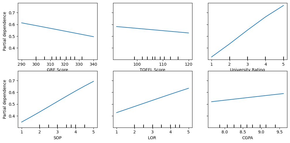
14.7.1. PDP, saturated model
It’s interesting that the PDP for GRE Score and TOEFL Score have negative slopes.
[117]:
from sklearn.inspection import PartialDependenceDisplay
import matplotlib.pyplot as plt

fig, ax = plt.subplots(figsize=(10, 5))

PartialDependenceDisplay.from_estimator(m_sat, X, X.columns, random_state=37, ax=ax, n_jobs=-1)

fig.tight_layout()
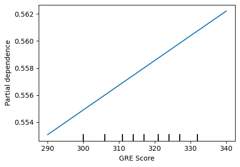
14.7.2. PDP, AUC-ROC + AUC-PR best model
[104]:
fig, ax = plt.subplots(figsize=(5, 3.5))

PartialDependenceDisplay.from_estimator(m_aps, X[['GRE Score']], ['GRE Score'], random_state=37, ax=ax, n_jobs=-1)

fig.tight_layout()
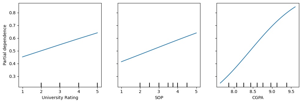
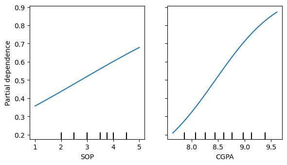
14.7.3. PDP, BSS best model
Note that CPGA looks curvilinear.
[107]:
fig, ax = plt.subplots(figsize=(10, 3.5))

PartialDependenceDisplay.from_estimator(m_bss, X[['University Rating', 'SOP', 'CGPA']], ['University Rating', 'SOP', 'CGPA'], random_state=37, ax=ax, n_jobs=-1)

fig.tight_layout()
14.7.4. PDP, LSS best model
[109]:
fig, ax = plt.subplots(figsize=(6, 3.5))

PartialDependenceDisplay.from_estimator(m_lss, X[['SOP', 'CGPA']], ['SOP', 'CGPA'], random_state=37, ax=ax, n_jobs=-1)

fig.tight_layout()
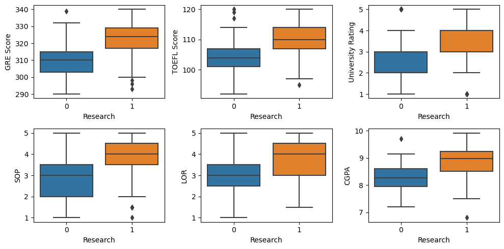
14.8. Box plots
The box plots of each feature by y (research) shows that students who have done research have higher values across all features.
[115]:
import seaborn as sns

fig, axes = plt.subplots(2, 3, figsize=(10, 5))

for c, ax in zip(X.columns, np.ravel(axes)):
    sns.boxplot(Xy, x='Research', y=c, ax=ax)

fig.tight_layout()
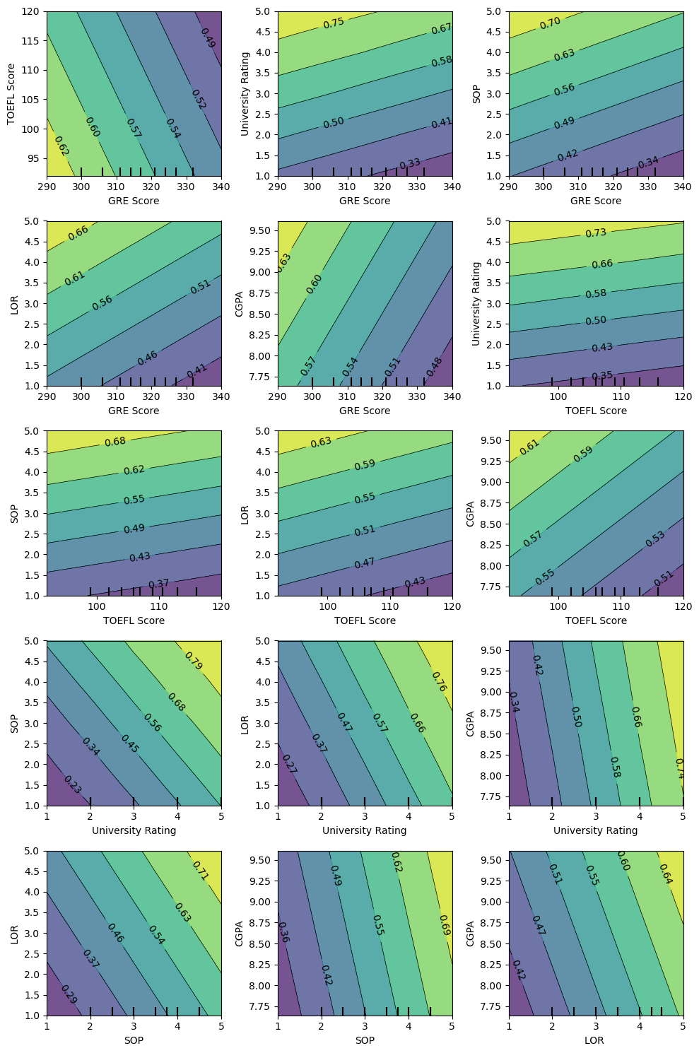
14.9. Two-way PDPs
Let’s look at some two-way PDP plots.
14.9.1. Two-way PDP, saturated model
[122]:
pairs = list(itertools.combinations(X.columns, 2))

fig, axes = plt.subplots(5, 3, figsize=(10, 15))

for p, ax in zip(pairs, np.ravel(axes)):
    PartialDependenceDisplay.from_estimator(m_sat, X, [p], random_state=37, ax=ax, n_jobs=-1)

fig.tight_layout()
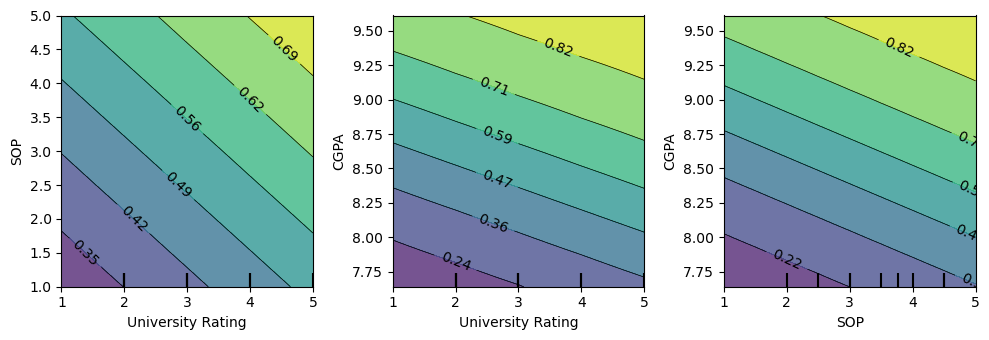
14.9.2. Two-way PDP, BSS best model
[150]:
pairs = list(itertools.combinations(['University Rating', 'SOP', 'CGPA'], 2))

fig, axes = plt.subplots(1, 3, figsize=(10, 3.5))

for p, ax in zip(pairs, np.ravel(axes)):
    PartialDependenceDisplay.from_estimator(m_bss, X[['University Rating', 'SOP', 'CGPA']], [p], random_state=37, ax=ax, n_jobs=-1)

fig.tight_layout()
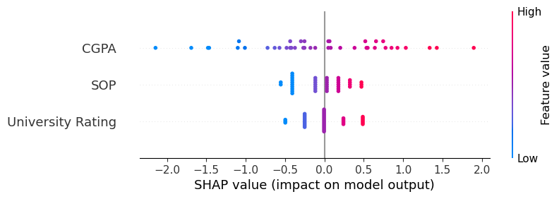
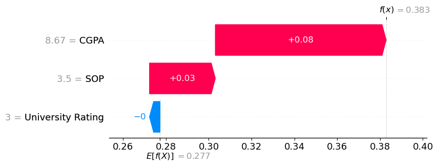
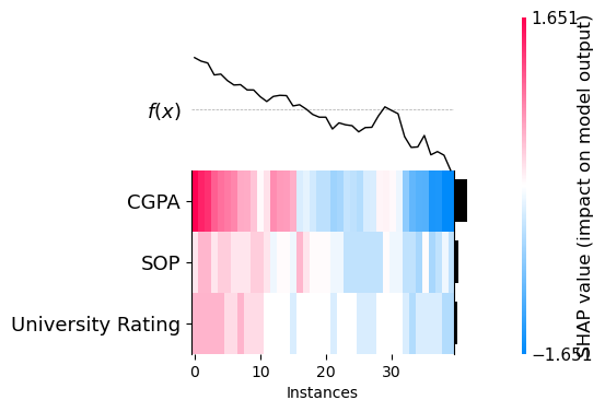
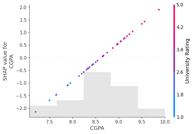
14.10. SHAP
Let’s look at the following SHAP plots.
[129]:
import shap

shap.initjs()

[130]:
explainer = shap.Explainer(m_bss, X_tr[['University Rating', 'SOP', 'CGPA']])
shap_values = explainer(X_te[['University Rating', 'SOP', 'CGPA']])
[131]:
shap.plots.beeswarm(shap_values)
No data for colormapping provided via 'c'. Parameters 'vmin', 'vmax' will be ignored
[164]:
shap.plots.force(shap_values[0])
[164]:
Have you run `initjs()` in this notebook? If this notebook was from another user you must also trust this notebook (File -> Trust notebook). If you are viewing this notebook on github the Javascript has been stripped for security. If you are using JupyterLab this error is because a JupyterLab extension has not yet been written.
[134]:
shap.plots.force(shap_values[1])
[134]:
Have you run `initjs()` in this notebook? If this notebook was from another user you must also trust this notebook (File -> Trust notebook). If you are viewing this notebook on github the Javascript has been stripped for security. If you are using JupyterLab this error is because a JupyterLab extension has not yet been written.
[144]:
shap.plots.force(shap_values[2])
[144]:
Have you run `initjs()` in this notebook? If this notebook was from another user you must also trust this notebook (File -> Trust notebook). If you are viewing this notebook on github the Javascript has been stripped for security. If you are using JupyterLab this error is because a JupyterLab extension has not yet been written.
[145]:
shap.plots.force(shap_values[3])
[145]:
Have you run `initjs()` in this notebook? If this notebook was from another user you must also trust this notebook (File -> Trust notebook). If you are viewing this notebook on github the Javascript has been stripped for security. If you are using JupyterLab this error is because a JupyterLab extension has not yet been written.
[161]:
shap.plots.waterfall(shap_values[0])
[167]:
shap.plots.heatmap(shap_values)
[169]:
shap.plots.scatter(shap_values[:, 'CGPA'], color=shap_values)
[170]:
shap.plots.scatter(shap_values[:, 'SOP'], color=shap_values)
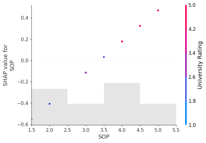
[171]:
shap.plots.scatter(shap_values[:, 'University Rating'], color=shap_values)
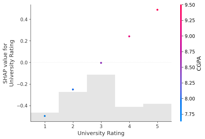
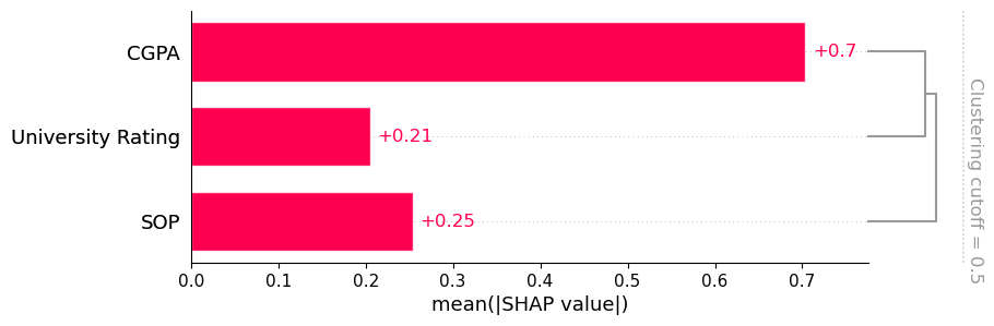
[174]:
shap.plots.bar(shap_values, clustering=shap.utils.hclust(X_te[['University Rating', 'SOP', 'CGPA']], y_te))
`early_stopping_rounds` in `fit` method is deprecated for better compatibility with scikit-learn, use `early_stopping_rounds` in constructor or`set_params` instead.