15. Kalman Filter, II

This notebook is a continuation of on KalmanFilter.NET [Bec18]. In this notebook, we focus on the Kalman Filter in one dimension.

15.1. Kalman Gain Equation

Before, the Kalman Gain \(K_n\) was held fixed or reduced over time by \(\dfrac{1}{n}\). Here \(K_n\) changes dynamically and depends on the meaurement device. To start, the Kalman Gain Equation \(K_n\) is defined as follows.

\(K_n = \dfrac{p_{n,n-1}}{p_{n,n-1} + r_n}\),

where

• \(p_{n,n-1}\) is the estimation uncertainty (variance)

• \(r_n\) is the measurement uncertainty (variance)

• \(0 \leq K_n \leq 1\)

The State Update Equation can be rewritten as follows.

\(\begin{array} \hat{x}_{n,n} & = & \hat{x}_{n,n-1} + K_n (z_n - \hat{x}_{n,n-1}) \\ & = & \hat{x}_{n,n-1} + K_n z_n - K_n \hat{x}_{n,n-1} \\ & = & \hat{x}_{n,n-1} - K_n \hat{x}_{n,n-1} + K_n z_n \\ & = & (1 - K_n) \hat{x}_{n,n-1} + K_n z_n\end{array}\)

When the State Update Equation is written as above, then

• \((1 - K_n)\) is the weight given to the estimate

• \(K_n\) is the weight given to the measurement

The Covariance Update Equation is given as follows.

\(p_{n,n} = (1 - K_n) p_{n,n-1}\)

The Covariance Extrapolation Equations for the position \(x\) and velocity \(v\) are give as follows.

• \(p^x_{n+1,n} = p^x_{n,n} + \Delta t^2 p^v_{n,n}\)

• \(p^v_{n+1,n} = p^v_{n,n}\)

15.2. Building height, estimation and measurement uncertainties

import pandas as pd

data = []

r = 25      # measurement uncertainty
x_ii = 60   # estimate
p_ii = 225  # estimate uncertainty

x_ji = x_ii # prediction
p_ji = p_ii # prediction uncertainty

Z = [48.54, 47.11, 55.01, 55.15, 49.89, 40.85, 46.72, 50.05, 51.27, 49.95]

for z_i in Z:
    K_i = p_ji / (p_ji + r)

    x_ii = x_ji + K_i * (z_i - x_ji)
    p_ii = (1 - K_i) * p_ji

    x_ji = x_ii
    p_ji = p_ii

    data.append({
        'K_i': K_i,
        'x_ii': x_ii,
        'p_ii': p_ii,
        'z_i': z_i,
        'r_i': r
    })

data = pd.DataFrame(data)
data.index = range(1, data.shape[0] + 1)
data

	K_i	x_ii	p_ii	z_i	r_i
1	0.900000	49.686000	22.500000	48.54	25
2	0.473684	48.465789	11.842105	47.11	25
3	0.321429	50.569286	8.035714	55.01	25
4	0.243243	51.683514	6.081081	55.15	25
5	0.195652	51.332609	4.891304	49.89	25
6	0.163636	49.617273	4.090909	40.85	25
7	0.140625	49.209844	3.515625	46.72	25
8	0.123288	49.313425	3.082192	50.05	25
9	0.109756	49.528171	2.743902	51.27	25
10	0.098901	49.569890	2.472527	49.95	25

import matplotlib.pyplot as plt

plt.style.use('ggplot')

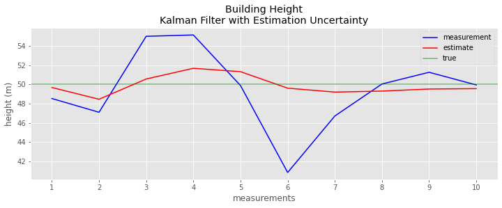
fig, ax = plt.subplots(figsize=(12, 4))

_ = data.z_i.plot(kind='line', ax=ax, color='blue', label='measurement')
_ = data.x_ii.plot(kind='line', ax=ax, color='red', label='estimate')
_ = ax.axhline(50, color='green', alpha=0.5, label='true')
_ = ax.set_xticks(range(1, data.shape[0] + 1))
_ = ax.set_xticklabels(data.index)
_ = ax.legend()
_ = ax.set_xlabel('measurements')
_ = ax.set_ylabel('height (m)')
_ = ax.set_title('Building Height\nKalman Filter with Estimation Uncertainty')

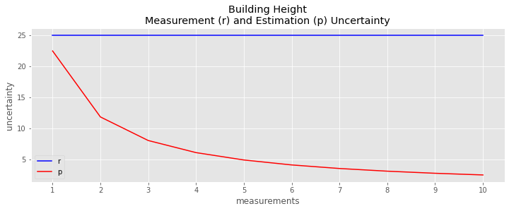
fig, ax = plt.subplots(figsize=(12, 4))

_ = data.r_i.plot(kind='line', ax=ax, color='blue', label='r')
_ = data.p_ii.plot(kind='line', ax=ax, color='red', label='p')
_ = ax.set_xticks(range(1, data.shape[0] + 1))
_ = ax.set_xticklabels(data.index)
_ = ax.legend()
_ = ax.set_xlabel('measurements')
_ = ax.set_ylabel('uncertainty')
_ = ax.set_title('Building Height\nMeasurement (r) and Estimation (p) Uncertainty')

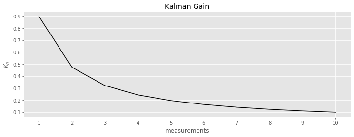
fig, ax = plt.subplots(figsize=(12, 4))

_ = data.K_i.plot(kind='line', ax=ax, color='black')
_ = ax.set_xticks(range(1, data.shape[0] + 1))
_ = ax.set_xticklabels(data.index)
_ = ax.set_xlabel('measurements')
_ = ax.set_ylabel(r'$K_n$')
_ = ax.set_title('Kalman Gain')