1. Bradley-Terry-Luce Model
For two items \(i\) and \(j\), the Bradley-Terry Model (or Bradley-Terry-Luce Model) BTM estimates the probability of \(i > j\) denoted as \(P(i > j)\). \(P(i > j)\) may be estimated as follows,
\(P(i > j) = \dfrac{p_i}{p_i + p_j}\)
where \(p_i\) is a positive real-valued scored assigned to the i-th item. The interpretation of \(i > j\) depends on the context and may mean
\(i\) comes before \(j\),
\(i\) wins over \(j\), or
\(i\) ranks higher than \(j\).
The goal of of BTM is to estimate each \(p_i\) for each i-th item, and then we can order these estimates in descending order which produces the ranking. Additionally, each pair \(p_i\) and \(p_j\) may then be used to compute \(P(i > j)\) as defined above.
There are many methods to estimate \(p_i\), and we will look at estimating these values in two ways:
through an iterative fashion like the EM Algorithm using a
n x ntable structure (where n is the number of items),through regression using a
m x ntable structure (where m is the number of head-to-head pairings and n is the number of items).
1.1. Dummy data
Here is data taken from Wikipedia. This data represents 4 teams: A, B, C, D. Each row is the number of times a team has beaten another one (as indicated by the column). So, for the first row, A has beaten B twice, A has not played C, and A has beaten D once. A team cannot play itself, and that is why the diagonal entries are missing.
[1]:
import pandas as pd
import numpy as np

df = pd.DataFrame({
    'A': [np.nan, 3, 0, 4],
    'B': [2, np.nan, 3, 0],
    'C': [0, 5, np.nan, 3],
    'D': [1, 0, 1, np.nan]
}, index=['A', 'B', 'C', 'D'])

df
[1]:
| A | B | C | D | |
|---|---|---|---|---|
| A | NaN | 2.0 | 0.0 | 1.0 |
| B | 3.0 | NaN | 5.0 | 0.0 |
| C | 0.0 | 3.0 | NaN | 1.0 |
| D | 4.0 | 0.0 | 3.0 | NaN |
Since there are 4 teams, we have to estimate 4 probabilities \(p_1\), \(p_2\), \(p_3\) and \(p_4\) corresponding to team A, B, C and D. The formula to estimate each \(p_i\) is as follows
\(p_i = \dfrac{W_i}{\sum_{j \neq i} \dfrac{w_{ij} + w_{ji}}{p_i + p_j}}\)
where
\(W_i\) is the total number of wins by the
i-thitem (sum across the rows),\(w_{ij}\) is the total number of times \(i\) beats \(j\),
\(w_{ji}\) is the total number of times \(j\) beats \(i\),
\(p_i\) is the current estimate of the
i-thitem, and\(p_j\) is the current estimate of the
j-thitem.
Initially, we must guess all \(p_i\), and in this case, we will set them all to 1. For example, \(p = [p_1, p_2, p_3, p_4] = [1, 1, 1, 1]\). We iterate many times to update \(p_i\) until some termination condition (either we have reached the max iterations or \(p\) has converged). The code below shows how to estimate \(p\).
[2]:
def get_estimate(i, p, df):
    get_prob = lambda i, j: np.nan if i == j else p.iloc[i] + p.iloc[j]
    n = df.iloc[i].sum()

    d_n = df.iloc[i] + df.iloc[:, i]
    d_d = pd.Series([get_prob(i, j) for j in range(len(p))], index=p.index)
    d = (d_n / d_d).sum()

    return n / d

def estimate_p(p, df):
    return pd.Series([get_estimate(i, p, df) for i in range(df.shape[0])], index=p.index)


def iterate(df, p=None, n=20, sorted=True):
    if p is None:
        p = pd.Series([1 for _ in range(df.shape[0])], index=list(df.columns))

    estimates = [p]

    for _ in range(n):
        p = estimate_p(p, df)
        p = p / p.sum()
        estimates.append(p)

    p = p.sort_values(ascending=False) if sorted else p
    return p, pd.DataFrame(estimates)

p, estimates = iterate(df, n=100)
Team D has the highest \(p_i\) and the ordering or ranking is D, B, C and A.
[3]:
p
[3]:
D    0.492133
B    0.226152
C    0.143022
A    0.138692
dtype: float64
We have also logged and traced the estimations and we can see that \(p\) has converged well before 100 iterations.
[4]:
estimates.tail()
[4]:
| A | B | C | D | |
|---|---|---|---|---|
| 96 | 0.138692 | 0.226152 | 0.143022 | 0.492133 |
| 97 | 0.138692 | 0.226152 | 0.143022 | 0.492133 |
| 98 | 0.138692 | 0.226152 | 0.143022 | 0.492133 |
| 99 | 0.138692 | 0.226152 | 0.143022 | 0.492133 |
| 100 | 0.138692 | 0.226152 | 0.143022 | 0.492133 |
1.2. 2021 NFL data
Let’s have some fun. We have download NFL data for the 2021 season up to November 25, 2021.
[5]:
def get_winner(r):
    if r.score1 > r.score2:
        return r.team1
    elif r.score1 < r.score2:
        return r.team2
    else:
        return np.nan

def get_loser(r):
    if r.score1 > r.score2:
        return r.team2
    elif r.score1 < r.score2:
        return r.team1
    else:
        return np.nan

nfl = pd.read_csv('./nfl/2021.csv')
nfl['team1'] = nfl['team1'].apply(lambda s: s.strip())
nfl['team2'] = nfl['team2'].apply(lambda s: s.strip())
nfl = nfl.drop_duplicates()
nfl['winner'] = nfl.apply(get_winner, axis=1)
nfl['loser'] = nfl.apply(get_loser, axis=1)

nfl.head()
[5]:
| team1 | team2 | score1 | score2 | week | winner | loser | |
|---|---|---|---|---|---|---|---|
| 0 | Cowboys | Buccaneers | 29 | 31 | 1 | Buccaneers | Cowboys |
| 1 | Eagles | Falcons | 32 | 6 | 1 | Eagles | Falcons |
| 2 | Chargers | Washington | 20 | 16 | 1 | Chargers | Washington |
| 3 | Steelers | Bills | 23 | 16 | 1 | Steelers | Bills |
| 4 | 49ers | Lions | 41 | 33 | 1 | 49ers | Lions |
We can transform the raw data into a table where each row corresponds to a team, and the columns tracks the number of wins and losses.
[6]:
import matplotlib.pyplot as plt

plt.style.use('ggplot')

w = nfl.winner.value_counts().sort_index()
l = nfl.loser.value_counts().sort_index()

wl_df = pd.DataFrame([w, l]).T.rename(columns={'winner': 'wins', 'loser': 'losses'})
wl_df = wl_df.fillna(0)
wl_df['n'] = wl_df.wins + wl_df.losses
wl_df
[6]:
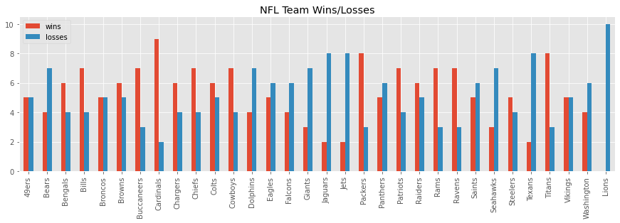
| wins | losses | n | |
|---|---|---|---|
| 49ers | 5.0 | 5.0 | 10.0 |
| Bears | 4.0 | 7.0 | 11.0 |
| Bengals | 6.0 | 4.0 | 10.0 |
| Bills | 7.0 | 4.0 | 11.0 |
| Broncos | 5.0 | 5.0 | 10.0 |
| Browns | 6.0 | 5.0 | 11.0 |
| Buccaneers | 7.0 | 3.0 | 10.0 |
| Cardinals | 9.0 | 2.0 | 11.0 |
| Chargers | 6.0 | 4.0 | 10.0 |
| Chiefs | 7.0 | 4.0 | 11.0 |
| Colts | 6.0 | 5.0 | 11.0 |
| Cowboys | 7.0 | 4.0 | 11.0 |
| Dolphins | 4.0 | 7.0 | 11.0 |
| Eagles | 5.0 | 6.0 | 11.0 |
| Falcons | 4.0 | 6.0 | 10.0 |
| Giants | 3.0 | 7.0 | 10.0 |
| Jaguars | 2.0 | 8.0 | 10.0 |
| Jets | 2.0 | 8.0 | 10.0 |
| Packers | 8.0 | 3.0 | 11.0 |
| Panthers | 5.0 | 6.0 | 11.0 |
| Patriots | 7.0 | 4.0 | 11.0 |
| Raiders | 6.0 | 5.0 | 11.0 |
| Rams | 7.0 | 3.0 | 10.0 |
| Ravens | 7.0 | 3.0 | 10.0 |
| Saints | 5.0 | 6.0 | 11.0 |
| Seahawks | 3.0 | 7.0 | 10.0 |
| Steelers | 5.0 | 4.0 | 9.0 |
| Texans | 2.0 | 8.0 | 10.0 |
| Titans | 8.0 | 3.0 | 11.0 |
| Vikings | 5.0 | 5.0 | 10.0 |
| Washington | 4.0 | 6.0 | 10.0 |
| Lions | 0.0 | 10.0 | 10.0 |
Here’s a visualization of the wins and losses per NFL team.
[7]:
_ = wl_df[['wins', 'losses']].plot(kind='bar', figsize=(15, 4), title='NFL Team Wins/Losses')
Now, we will transform the raw data to a n x n matrix, where n is the number of NFL teams (32). Each row will represent a team, and each column in a row will represent how many times the team in the row has beaten the team in the column.
[8]:
teams = sorted(list(set(nfl.team1) | set(nfl.team2)))
t2i = {t: i for i, t in enumerate(teams)}

df = nfl\
    .groupby(['winner', 'loser'])\
    .agg('count')\
    .drop(columns=['team2', 'score1', 'score2'])\
    .rename(columns={'team1': 'n'})\
    .reset_index()
df['r'] = df['winner'].apply(lambda t: t2i[t])
df['c'] = df['loser'].apply(lambda t: t2i[t])

n_teams = len(teams)
mat = np.zeros([n_teams, n_teams])

for _, r in df.iterrows():
    mat[r.r, r.c] = r.n

df = pd.DataFrame(mat, columns=teams, index=teams)

df.head()
[8]:
| 49ers | Bears | Bengals | Bills | Broncos | Browns | Buccaneers | Cardinals | Chargers | Chiefs | ... | Raiders | Rams | Ravens | Saints | Seahawks | Steelers | Texans | Titans | Vikings | Washington | |
|---|---|---|---|---|---|---|---|---|---|---|---|---|---|---|---|---|---|---|---|---|---|
| 49ers | 0.0 | 1.0 | 0.0 | 0.0 | 0.0 | 0.0 | 0.0 | 0.0 | 0.0 | 0.0 | ... | 0.0 | 1.0 | 0.0 | 0.0 | 0.0 | 0.0 | 0.0 | 0.0 | 0.0 | 0.0 |
| Bears | 0.0 | 0.0 | 1.0 | 0.0 | 0.0 | 0.0 | 0.0 | 0.0 | 0.0 | 0.0 | ... | 1.0 | 0.0 | 0.0 | 0.0 | 0.0 | 0.0 | 0.0 | 0.0 | 0.0 | 0.0 |
| Bengals | 0.0 | 0.0 | 0.0 | 0.0 | 0.0 | 0.0 | 0.0 | 0.0 | 0.0 | 0.0 | ... | 1.0 | 0.0 | 1.0 | 0.0 | 0.0 | 1.0 | 0.0 | 0.0 | 1.0 | 0.0 |
| Bills | 0.0 | 0.0 | 0.0 | 0.0 | 0.0 | 0.0 | 0.0 | 0.0 | 0.0 | 1.0 | ... | 0.0 | 0.0 | 0.0 | 1.0 | 0.0 | 0.0 | 1.0 | 0.0 | 0.0 | 1.0 |
| Broncos | 0.0 | 0.0 | 0.0 | 0.0 | 0.0 | 0.0 | 0.0 | 0.0 | 0.0 | 0.0 | ... | 0.0 | 0.0 | 0.0 | 0.0 | 0.0 | 0.0 | 0.0 | 0.0 | 0.0 | 1.0 |
5 rows × 32 columns
Now, we can estimate \(p\).
[9]:
p, estimates = iterate(df, n=100)
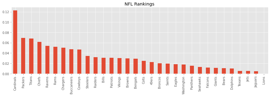
As you can see, the Cardinals is the top team. The Packers and Titans are very close to each other. The worst team is the Lions.
[10]:
p
[10]:
Cardinals     0.122781
Packers       0.069247
Titans        0.068104
Chiefs        0.061767
Ravens        0.053967
Rams          0.052400
Chargers      0.050219
Buccaneers    0.047603
Cowboys       0.046897
Steelers      0.034552
Raiders       0.031772
Bills         0.030949
Patriots      0.030948
Vikings       0.030064
Browns        0.029378
Bengals       0.029071
Colts         0.024912
49ers         0.022290
Broncos       0.019892
Saints        0.019743
Eagles        0.018422
Washington    0.017573
Panthers      0.015306
Seahawks      0.012831
Falcons       0.011700
Giants        0.011220
Bears         0.010692
Dolphins      0.009925
Texans        0.005485
Jets          0.005413
Jaguars       0.004875
Lions         0.000000
dtype: float64
Here’s a bar plot of \(p\) sorted descendingly.
[11]:
_ = p.plot(kind='bar', figsize=(15, 4), title='NFL Rankings')
1.3. 2021 NBA data
We can also get NBA data for the 2021 season from October 19, 2021 to November 24, 2021.
[12]:
def get_winner(r):
    if r.a_score > r.h_score:
        return r.a_team
    elif r.a_score < r.h_score:
        return r.h_team
    else:
        return np.nan

def get_loser(r):
    if r.a_score > r.h_score:
        return r.h_team
    elif r.a_score < r.h_score:
        return r.a_team
    else:
        return np.nan

nba = pd.read_csv('./nba/2021.csv')
nba['a_team'] = nba['a_team'].apply(lambda s: s.strip())
nba['h_team'] = nba['h_team'].apply(lambda s: s.strip())
nba['winner'] = nba.apply(get_winner, axis=1)
nba['loser'] = nba.apply(get_loser, axis=1)

nba.head()
[12]:
| a_team | h_team | a_score | h_score | preseason | winner | loser | |
|---|---|---|---|---|---|---|---|
| 0 | Nets | Lakers | 123 | 97 | True | Nets | Lakers |
| 1 | 76ers | Raptors | 107 | 123 | True | Raptors | 76ers |
| 2 | Hawks | Heat | 99 | 125 | True | Heat | Hawks |
| 3 | Magic | Celtics | 97 | 98 | True | Celtics | Magic |
| 4 | Pelicans | Timberwolves | 114 | 117 | True | Timberwolves | Pelicans |
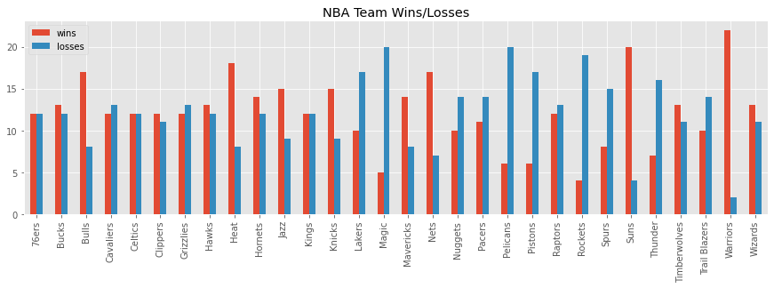
Here’s the number of wins and losses per team.
[13]:
w = nba.winner.value_counts().sort_index()
l = nba.loser.value_counts().sort_index()

wl_df = pd.DataFrame([w, l]).T.rename(columns={'winner': 'wins', 'loser': 'losses'})
wl_df = wl_df.fillna(0)
wl_df['n'] = wl_df.wins + wl_df.losses
wl_df
[13]:
| wins | losses | n | |
|---|---|---|---|
| 76ers | 12 | 12 | 24 |
| Bucks | 13 | 12 | 25 |
| Bulls | 17 | 8 | 25 |
| Cavaliers | 12 | 13 | 25 |
| Celtics | 12 | 12 | 24 |
| Clippers | 12 | 11 | 23 |
| Grizzlies | 12 | 13 | 25 |
| Hawks | 13 | 12 | 25 |
| Heat | 18 | 8 | 26 |
| Hornets | 14 | 12 | 26 |
| Jazz | 15 | 9 | 24 |
| Kings | 12 | 12 | 24 |
| Knicks | 15 | 9 | 24 |
| Lakers | 10 | 17 | 27 |
| Magic | 5 | 20 | 25 |
| Mavericks | 14 | 8 | 22 |
| Nets | 17 | 7 | 24 |
| Nuggets | 10 | 14 | 24 |
| Pacers | 11 | 14 | 25 |
| Pelicans | 6 | 20 | 26 |
| Pistons | 6 | 17 | 23 |
| Raptors | 12 | 13 | 25 |
| Rockets | 4 | 19 | 23 |
| Spurs | 8 | 15 | 23 |
| Suns | 20 | 4 | 24 |
| Thunder | 7 | 16 | 23 |
| Timberwolves | 13 | 11 | 24 |
| Trail Blazers | 10 | 14 | 24 |
| Warriors | 22 | 2 | 24 |
| Wizards | 13 | 11 | 24 |
[14]:
_ = wl_df[['wins', 'losses']].plot(kind='bar', figsize=(15, 4), title='NBA Team Wins/Losses')
We will transform the data to a n x n matrix (n=30) again.
[15]:
teams = sorted(list(set(nba.a_team) | set(nba.h_team)))
t2i = {t: i for i, t in enumerate(teams)}

df = nba\
    .groupby(['winner', 'loser'])\
    .agg('count')\
    .drop(columns=['h_team', 'a_score', 'h_score'])\
    .rename(columns={'a_team': 'n'})\
    .reset_index()
df['r'] = df['winner'].apply(lambda t: t2i[t])
df['c'] = df['loser'].apply(lambda t: t2i[t])

n_teams = len(teams)
mat = np.zeros([n_teams, n_teams])

for _, r in df.iterrows():
    mat[r.r, r.c] = r.n

df = pd.DataFrame(mat, columns=teams, index=teams)

df.shape
[15]:
(30, 30)
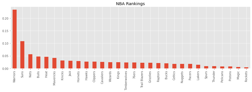
Below is \(p\) and the rankings. The Warriors are the highest ranked team, followed by the Suns. The worst teams are the Magic and Rockets.
[16]:
p, estimates = iterate(df, n=100)
p
[16]:
Warriors         0.234286
Suns             0.108259
Nets             0.056412
Bulls            0.047578
Heat             0.046572
Mavericks        0.041772
Knicks           0.031417
Jazz             0.030731
Hornets          0.028883
Hawks            0.027017
Clippers         0.026891
Cavaliers        0.025853
Wizards          0.024828
Kings            0.024613
Timberwolves     0.023990
76ers            0.023138
Trail Blazers    0.022861
Grizzlies        0.022233
Raptors          0.020807
Bucks            0.020189
Celtics          0.018374
Nuggets          0.018167
Pacers           0.018018
Lakers           0.014244
Spurs            0.008889
Thunder          0.008728
Pelicans         0.008001
Pistons          0.007736
Magic            0.005067
Rockets          0.004447
dtype: float64
[17]:
_ = p.plot(kind='bar', figsize=(15, 4), title='NBA Rankings')
1.4. Logistic Regression
The iterative approach is not the only way to estimate \(p\), and we can use logistic regression. However, the data structure is no longer a n x n matrix, but a m x n matrix, where m is the number of games played and n is the number of teams.
The m x n design matrix has some nuances.
Each row represents a game.
Each row is sparse (mostly zeros).
Since there are only 2 teams per game, only 2 entries per row will be non-zero. The column corresponding to the home team will be 1 and the column corresponding to the away team will be -1.
The dependent variable y will be set to 1 if the home team wins and 0 otherwise.
[18]:
def get_vector(r):
    y = {'y': 1 if r.h_score > r.a_score else 0}

    v = {t: 0 for t in teams}
    v[r.a_team] = -1
    v[r.h_team] = 1

    return {**y, **v}

X = pd.DataFrame(list(nba.apply(get_vector, axis=1)))
y = X.y
X = X[[c for c in X.columns if c != 'y']]

X.head()
[18]:
| 76ers | Bucks | Bulls | Cavaliers | Celtics | Clippers | Grizzlies | Hawks | Heat | Hornets | ... | Pistons | Raptors | Rockets | Spurs | Suns | Thunder | Timberwolves | Trail Blazers | Warriors | Wizards | |
|---|---|---|---|---|---|---|---|---|---|---|---|---|---|---|---|---|---|---|---|---|---|
| 0 | 0 | 0 | 0 | 0 | 0 | 0 | 0 | 0 | 0 | 0 | ... | 0 | 0 | 0 | 0 | 0 | 0 | 0 | 0 | 0 | 0 |
| 1 | -1 | 0 | 0 | 0 | 0 | 0 | 0 | 0 | 0 | 0 | ... | 0 | 1 | 0 | 0 | 0 | 0 | 0 | 0 | 0 | 0 |
| 2 | 0 | 0 | 0 | 0 | 0 | 0 | 0 | -1 | 1 | 0 | ... | 0 | 0 | 0 | 0 | 0 | 0 | 0 | 0 | 0 | 0 |
| 3 | 0 | 0 | 0 | 0 | 1 | 0 | 0 | 0 | 0 | 0 | ... | 0 | 0 | 0 | 0 | 0 | 0 | 0 | 0 | 0 | 0 |
| 4 | 0 | 0 | 0 | 0 | 0 | 0 | 0 | 0 | 0 | 0 | ... | 0 | 0 | 0 | 0 | 0 | 0 | 1 | 0 | 0 | 0 |
5 rows × 30 columns
Now we can use logistic regression on the transformed data. Note here we use lasso as the penalty.
[19]:
from sklearn.linear_model import LogisticRegression

l1_model = LogisticRegression(penalty='l1', solver='liblinear', fit_intercept=True)
l1_model.fit(X, y)
q = sorted(list(zip(X.columns, l1_model.coef_[0])), key=lambda tup: tup[1], reverse=True)
q = pd.Series([c for _, c in q], index=[t for t, _ in q])
q
[19]:
Warriors         1.791846
Suns             1.272234
Nets             0.677548
Heat             0.604793
Bulls            0.502055
Mavericks        0.415153
Knicks           0.130163
Jazz             0.116884
Hornets          0.071465
76ers            0.000000
Bucks            0.000000
Cavaliers        0.000000
Celtics          0.000000
Clippers         0.000000
Grizzlies        0.000000
Hawks            0.000000
Kings            0.000000
Raptors          0.000000
Timberwolves     0.000000
Trail Blazers    0.000000
Wizards          0.000000
Pacers          -0.057087
Nuggets         -0.087430
Lakers          -0.324553
Spurs           -0.661807
Thunder         -0.747753
Pistons         -0.856171
Pelicans        -0.897271
Magic           -1.202521
Rockets         -1.266441
dtype: float64
We can also use logistic regression with ridge regularization.
[20]:
l2_model = LogisticRegression(penalty='l2', solver='liblinear', fit_intercept=True)
l2_model.fit(X, y)
r = sorted(list(zip(X.columns, l2_model.coef_[0])), key=lambda tup: tup[1], reverse=True)
r = pd.Series([c for _, c in r], index=[t for t, _ in r])
r
[20]:
Warriors         1.586253
Suns             1.226357
Nets             0.745499
Heat             0.702808
Bulls            0.595838
Mavericks        0.534591
Knicks           0.290732
Jazz             0.280654
Hornets          0.223962
Hawks            0.156548
Wizards          0.134589
Cavaliers        0.074674
Kings            0.045510
76ers            0.032626
Timberwolves     0.026530
Raptors          0.012512
Clippers        -0.004593
Bucks           -0.028013
Grizzlies       -0.070541
Celtics         -0.088156
Trail Blazers   -0.092386
Pacers          -0.156770
Nuggets         -0.225596
Lakers          -0.433530
Spurs           -0.704429
Thunder         -0.785490
Pistons         -0.867906
Pelicans        -0.869052
Magic           -1.130543
Rockets         -1.212677
dtype: float64
1.5. Rankings
Let’s compare the rankings estimated by these different procedures.
p: iterative
q: Logistic Regression L1
r: Logistic Regression L2
[21]:
rank_df = pd.DataFrame([p, q, r]).T.rename(columns={0: 'p', 1: 'q', 2: 'r'})
rank_df
[21]:
| p | q | r | |
|---|---|---|---|
| Warriors | 0.234286 | 1.791846 | 1.586253 |
| Suns | 0.108259 | 1.272234 | 1.226357 |
| Nets | 0.056412 | 0.677548 | 0.745499 |
| Bulls | 0.047578 | 0.502055 | 0.595838 |
| Heat | 0.046572 | 0.604793 | 0.702808 |
| Mavericks | 0.041772 | 0.415153 | 0.534591 |
| Knicks | 0.031417 | 0.130163 | 0.290732 |
| Jazz | 0.030731 | 0.116884 | 0.280654 |
| Hornets | 0.028883 | 0.071465 | 0.223962 |
| Hawks | 0.027017 | 0.000000 | 0.156548 |
| Clippers | 0.026891 | 0.000000 | -0.004593 |
| Cavaliers | 0.025853 | 0.000000 | 0.074674 |
| Wizards | 0.024828 | 0.000000 | 0.134589 |
| Kings | 0.024613 | 0.000000 | 0.045510 |
| Timberwolves | 0.023990 | 0.000000 | 0.026530 |
| 76ers | 0.023138 | 0.000000 | 0.032626 |
| Trail Blazers | 0.022861 | 0.000000 | -0.092386 |
| Grizzlies | 0.022233 | 0.000000 | -0.070541 |
| Raptors | 0.020807 | 0.000000 | 0.012512 |
| Bucks | 0.020189 | 0.000000 | -0.028013 |
| Celtics | 0.018374 | 0.000000 | -0.088156 |
| Nuggets | 0.018167 | -0.087430 | -0.225596 |
| Pacers | 0.018018 | -0.057087 | -0.156770 |
| Lakers | 0.014244 | -0.324553 | -0.433530 |
| Spurs | 0.008889 | -0.661807 | -0.704429 |
| Thunder | 0.008728 | -0.747753 | -0.785490 |
| Pelicans | 0.008001 | -0.897271 | -0.869052 |
| Pistons | 0.007736 | -0.856171 | -0.867906 |
| Magic | 0.005067 | -1.202521 | -1.130543 |
| Rockets | 0.004447 | -1.266441 | -1.212677 |
Is there high correlation between these ranking approaches?
[22]:
rank_df.corr()
[22]:
| p | q | r | |
|---|---|---|---|
| p | 1.000000 | 0.816128 | 0.774388 |
| q | 0.816128 | 1.000000 | 0.988253 |
| r | 0.774388 | 0.988253 | 1.000000 |
1.6. Prediction
Once we have the logistic models, we can make predictions about winning. Below, we compute Suns vs Warriors when the game is played in Phoenix or The Bay. Note the asymmetry in the prediction; when the Suns play the Warriors at home, they have a 45% chance of winning (L1 model), but when the Suns play the Warriors as the away team, they have 31% (1 - 0.69) chance of winning.
[23]:
def get_vector(a_team, h_team):
    v = {t: 0 for t in teams}
    v[a_team] = -1
    v[h_team] = 1

    return pd.DataFrame([v])

print('@Suns vs Warriors')
g = get_vector('Warriors', 'Suns')
print(l1_model.predict_proba(g)[0, 1], l2_model.predict_proba(g)[0, 1])

print('Suns vs @Warriors')
g = get_vector('Suns', 'Warriors')
print(l1_model.predict_proba(g)[0, 1], l2_model.predict_proba(g)[0, 1])
@Suns vs Warriors
0.4510242710808479 0.49480517993288603
Suns vs @Warriors
0.6990317451260665 0.66796872013519
[24]:
params = np.asarray([rank_df.loc['Warriors'].p, rank_df.loc['Suns'].p])

e = np.exp(params - np.max(params))
e / e.sum(axis=0)
[24]:
array([0.53146502, 0.46853498])