5. Neural Networks, Gradient Descent

In this notebook, we show how to use neural networks (NNs) with PyTorch to solve a linear regression problem using different gradient descent methods. The three gradient descent methods we will look at are

• batch gradient descent,

• stochastic gradient descent, and

• mini-batch gradient descent.

If you recall, ordinary least square (OLS) regression problems of the form \(y = \beta + w_1 x_1 + \ldots + w_n x_n\) are solved through maximum likelihood methods. The weights, \(w = \{w_1, \ldots, w_n\}\), of a regression model are estimated through a loss function. Initially, we guess what the weights are, and then we make predictions \(\hat{y}\) based on the weights. The predictions \(\hat{y}\) will differ from the true values \(y\). The loss function is often written as follows \(L(y, \hat{y}) = (y - \hat{y})^2\). The partial derivative of the loss function (with respect to the weights) helps us adjust the weights in direction (negative or positive direction) and magnitude (how much do we move). Typically, the weights are adjusted as follows.

\(w^{*}_{j} = w_j - \alpha \frac{\partial L}{\partial w_j}\)

where

• \(w^{*}_{j}\) is the j-th new weight

• \(w_j\) is the j-th current weight

• \(\alpha\) is the learning rate

• \(\frac{\partial L}{\partial w_j}\) is the partial derivative of the loss function \(L\) with respect to the weight \(w_j\)

There are many ways to actually use the loss function and thus, errors, to adjust the weights.

• We can feed one example \(x = \{ x_1, \ldots, x_n \}\) to the model to get a prediction \(\hat{y}\), compute the error (loss), and then use the error to adjust the weights. Typically, we want to randomize the inputs \(x\) before feeding them one at a time to the model. We feed one example at a time until we run out of examples. This approach is called stochastic gradient descent.

• We can feed all examples to the model to get a vector of predictions, compute the average error, and then use this average error to adjust the weights. This approach is called batch gradient descent.

• We can feed a small number of examples to the model, compute the corresponding average error, and then use this average error to adjust the weights. Each of these small number of examples we feed into the model are called batches, and there are many ways to decide the size of the batch. We feed the model as many batches as we have until we run out of examples. This approach is called mini-batch gradient descent.

After we iterate over all examples, no matter the method (batch, stochastic, or mini-batch), this completion is termed an epoch; meaning, in one epoch, we have used all the training examples to adjust the weights. As you will see below, we need to run through many epochs when using NNs to learn the weights for a OLS regression model. All the NNs shown below will only have 2 layers, an input and output layer; so, the NN architectures are the same (identical). The difference is with training them through batch, stochastic, or mini-batch gradient descent.

5.1. Simulate data

Let’s simulate our data to following the equation \(y = 5.0 + w_1 x_1 + \epsilon\), where

• \(x_1 \sim \mathcal{N}(2, 1)\), \(x_1\) is sampled from a normal distribution of mean 2 and 1 standard deviation

• \(\epsilon \sim \mathcal{N}(0, 1)\), \(\epsilon\) is the error term and sampled from a normal distribution of mean 0 and 1 standard deviation

• \(y \sim \mathcal{N}(5.0 + w_1 x_1)\), \(y\) is sampled from a normal distribution of mean \(5.0 + w_1 x_1\) and 1 standard deviation

Note that we sampled 1,000 \(x, y\) pairs. Our matrix to represent the input values \(x\), however, has 2 columns; the first column represents the bias and all its values are 1; the second column represents the sampled \(x\). Note also that once we have our data, we need to convert them to PyTorch tensors.

%matplotlib inline
import numpy as np
import pandas as pd
import matplotlib.pylab as plt
import torch
import torch.nn as nn
from torch import optim
from numpy.random import normal
from sklearn.metrics import r2_score

np.random.seed(37)
torch.manual_seed(37)
torch.backends.cudnn.deterministic = True
torch.backends.cudnn.benchmark = False

device = torch.device('cuda') if torch.cuda.is_available() else torch.device('cpu')

n = 1000
X = np.hstack([
        np.ones(n).reshape(n, 1),
        normal(2.0, 1.0, n).reshape(n, 1)
    ])
y = normal(5.0 + 2.0 * X[:, 1], 1, n).reshape(n, 1) + normal(0, 1, n).reshape(n, 1)

X = torch.from_numpy(X).type(torch.FloatTensor).to(device)
y = torch.from_numpy(y).type(torch.FloatTensor).to(device)

print('X', X.shape, X.device)
print('y', y.shape, y.device)

X torch.Size([1000, 2]) cuda:0
y torch.Size([1000, 1]) cuda:0

5.2. Gradient descent

Here, we will define a 2 layers NN architecture, and apply the different gradient descent approaches. Note that we keep track of the losses and plot them out. We also estimated \(R^2\) value for each model resulting from each of the approaches. Finally, we use Scikit-Learn’s LinearRegression model to estimate the weights as well for a sanity check.

def plot_loss(loss_trace, title='Loss over epochs'):
    loss_df = pd.DataFrame(loss_trace, columns=['epoch', 'loss'])
    fig, ax = plt.subplots(1, 1, figsize=(15, 5))
    plt.plot(loss_df['epoch'], loss_df['loss'])
    ax.set_title(title)
    ax.set_xlabel('epoch')
    ax.set_ylabel('loss')

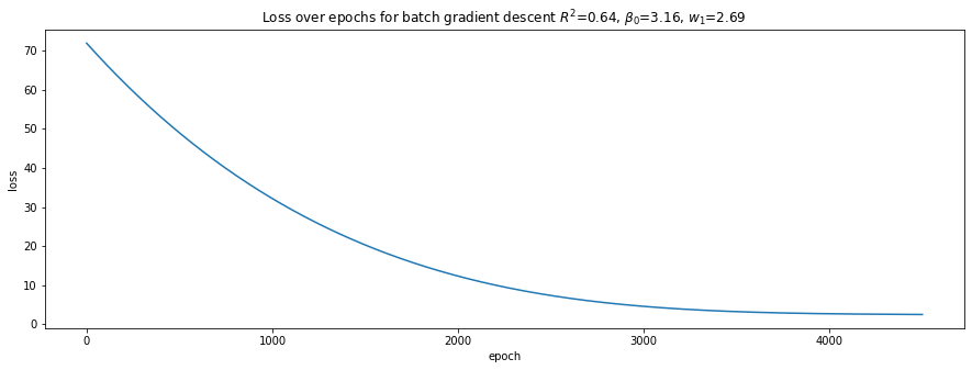
5.2.1. Batch gradient descent

model = torch.nn.Sequential(
    torch.nn.Linear(2, 1, bias=False)
)
model = model.to(device)
model.train()

loss_fn = torch.nn.MSELoss(reduction='mean')
learning_rate = 1e-3
optimizer = torch.optim.Adam(model.parameters(), lr=learning_rate)
loss_trace = []

for epoch in range(4500):
    optimizer.zero_grad()

    with torch.set_grad_enabled(True):
        y_pred = model(X)

        loss = loss_fn(y_pred, y)
        loss_trace.append((epoch, loss.item()))

        loss.backward()
        optimizer.step()

model.eval()
r2 = r2_score(model(X).cpu().detach().numpy(), y.cpu().detach().numpy())
b0 = model[0].weight[0, 0]
w1 = model[0].weight[0, 1]
plot_loss(loss_trace, r'Loss over epochs for batch gradient descent $R^2$={:.2f}, $\beta_0$={:.2f}, $w_1$={:.2f}'.format(r2, b0, w1))

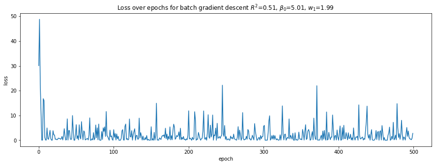
5.2.2. Stochastic gradient descent

model = torch.nn.Sequential(
    torch.nn.Linear(2, 1, bias=False)
)
model = model.to(device)
model.train()

loss_fn = torch.nn.MSELoss(reduction='mean')
learning_rate = 1e-3
optimizer = torch.optim.Adam(model.parameters(), lr=learning_rate)
loss_trace = []

for epoch in range(500):
    indices = list(range(n))
    np.random.shuffle(indices)

    for i in indices:
        optimizer.zero_grad()

        with torch.set_grad_enabled(True):
            y_pred = model(X[i])
            loss = loss_fn(y_pred, y[i])

            loss.backward()
            optimizer.step()

    loss_trace.append((epoch, loss.item()))

model.eval()
r2 = r2_score(model(X).cpu().detach().numpy(), y.cpu().detach().numpy())
b0 = model[0].weight[0, 0]
w1 = model[0].weight[0, 1]
plot_loss(loss_trace, r'Loss over epochs for batch gradient descent $R^2$={:.2f}, $\beta_0$={:.2f}, $w_1$={:.2f}'.format(r2, b0, w1))

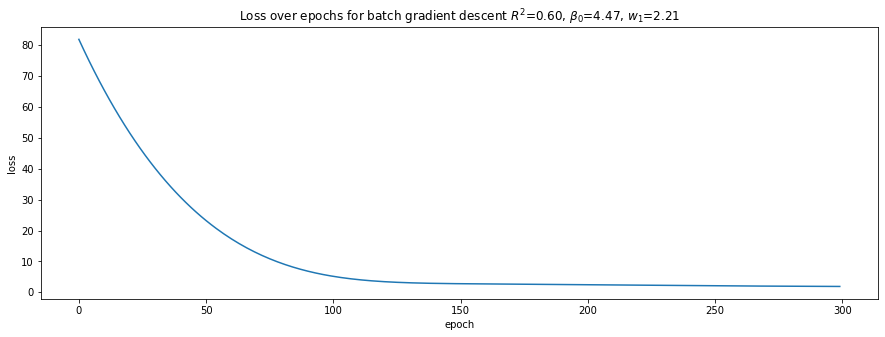
5.2.3. Mini-batch gradient descent

model = torch.nn.Sequential(
    torch.nn.Linear(2, 1, bias=False)
)
model = model.to(device)
model.train()

loss_fn = torch.nn.MSELoss(reduction='mean')
learning_rate = 1e-3
optimizer = torch.optim.Adam(model.parameters(), lr=learning_rate)
loss_trace = []

for epoch in range(300):
    start = 0
    batch_size = 32
    indices = list(range(n))

    while True:
        optimizer.zero_grad()

        stop = start + batch_size
        if stop >= n:
            stop = n

        with torch.set_grad_enabled(True):
            y_pred = model(X[indices])
            loss = loss_fn(y_pred, y[indices])

            loss.backward()
            optimizer.step()

        start += batch_size
        if start >= n:
            break

    loss_trace.append((epoch, loss.item()))

model.eval()
r2 = r2_score(model(X).cpu().detach().numpy(), y.cpu().detach().numpy())
b0 = model[0].weight[0, 0]
w1 = model[0].weight[0, 1]
plot_loss(loss_trace, r'Loss over epochs for batch gradient descent $R^2$={:.2f}, $\beta_0$={:.2f}, $w_1$={:.2f}'.format(r2, b0, w1))

5.2.4. Verify with Scikit-Learn Linear Model

from sklearn import linear_model

model = linear_model.LinearRegression(fit_intercept=False)
model.fit(X.cpu().detach().numpy(), y.cpu().detach().numpy())
print(model.coef_)
print(r2_score(model.predict(X.cpu().detach().numpy()), y.cpu().detach().numpy()))

[[5.0051513 1.9844328]]
0.5143197026642107

5.2.5. Summary of results

Here are some things to note.

• Batch gradient descent takes many more epochs (4,500) to learn the weights and converge. Mini-batch gradient descent takes only 300 epochs, and stochastic gradient descent takes 500 epochs.

• Batch and mini-batch gradient descents’ losses over epochs are smooth while stochastic gradient descent bounces up and down. This observation is no doubt related to randomization of the data.

• Stochastic gradient descent and Scikit-Learn’s LinearRegression learn the intercept and weight that are closest to the model’s true parameters, however, their \(R^2\) are not the highest, and, in fact, are the lowest.

• The NN learned through batch gradient descent has the highest \(R^2\) value, though the intercept and weight do not really resemble the model’s true parameters. Obviously, we have over-fitted our model.

5.2.6. Using DataLoader to control batch sizes

You can implement batch, stochastic, and mini-batch gradient descent using the DataLoader class. In the examples above, we manually controlled for batch sizes, however, with DataLoader, you can set the batch_size and shuffle properties to mimic the type of gradient descent you want.

• batch_size = n and shuffle = False indicates batch gradient descent

• batch_size = 1 and shuffle = True indicates stochastic gradient descent

• batch_size = k and shuffle = False indicates mini-batch gradient descent (where k << n)

The example below shows how we may use DataLoader to use minii-batch gradient descent.

import torch.utils.data as Data

loader = Data.DataLoader(
    dataset=Data.TensorDataset(X, y),
    batch_size=32,
    shuffle=True
)

model = torch.nn.Sequential(
    torch.nn.Linear(2, 1, bias=False)
)
model = model.to(device)
model.train()

loss_fn = torch.nn.MSELoss(reduction='mean')
learning_rate = 1e-3
optimizer = torch.optim.Adam(model.parameters(), lr=learning_rate)
loss_trace = []

for epoch in range(300):
    for step, (batch_x, batch_y) in enumerate(loader):
        optimizer.zero_grad()

        with torch.set_grad_enabled(True):
            y_pred = model(batch_x)
            loss = loss_fn(y_pred, batch_y)

            loss.backward()
            optimizer.step()
    loss_trace.append((epoch, loss.item()))

model.eval()
r2 = r2_score(model(X).cpu().detach().numpy(), y.cpu().detach().numpy())
b0 = model[0].weight[0, 0]
w1 = model[0].weight[0, 1]
plot_loss(loss_trace, r'Loss over epochs for mini-batch gradient descent $R^2$={:.2f}, $\beta_0$={:.2f}, $w_1$={:.2f}'.format(r2, b0, w1))

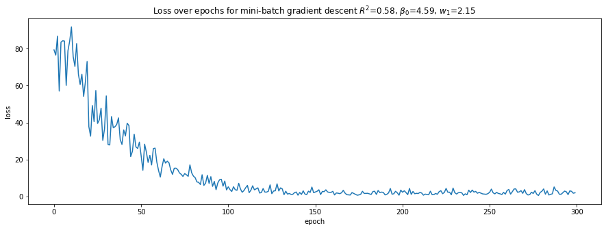
5.2.7. Having fun with more than 3 layers and mini-batch gradient descent

Here, we try to have fun and define 3 layers: 1 input, 1 hidden, and 1 output layer. Note that we switch over to using PyTorch’s Module to define the NN architecture. Note the results are not that great; hint, it is not easy to architect a NN.

class Net(torch.nn.Module):
    def __init__(self, n_feature, n_hidden, n_output):
        super(Net, self).__init__()
        self.hidden = torch.nn.Linear(n_feature, n_hidden, bias=False)
        self.predict = torch.nn.Linear(n_hidden, n_output, bias=False)

    def forward(self, x):
        x = torch.sigmoid(self.hidden(x))
        x = self.predict(x)
        return x

loader = Data.DataLoader(
    dataset=Data.TensorDataset(X, y),
    batch_size=32,
    shuffle=True
)

model = Net(n_feature=2, n_hidden=2, n_output=1)
model = model.to(device)
model.train()

loss_fn = torch.nn.MSELoss(reduction='mean')
learning_rate = 1e-3
optimizer = torch.optim.Adam(model.parameters(), lr=learning_rate)
loss_trace = []

for epoch in range(1000):
    for step, (batch_x, batch_y) in enumerate(loader):
        optimizer.zero_grad()

        with torch.set_grad_enabled(True):
            y_pred = model(batch_x)
            loss = loss_fn(y_pred, batch_y)

            loss.backward()
            optimizer.step()
    loss_trace.append((epoch, loss.item()))

model.eval()
r2 = r2_score(model(X).cpu().detach().numpy(), y.cpu().detach().numpy())
b0 = model.predict.weight[0, 0].cpu().detach().numpy()
w1 = model.predict.weight[0, 1].cpu().detach().numpy()
plot_loss(loss_trace, r'Loss over epochs for mini-batch gradient descent $R^2$={:.2f}, $\beta_0$={:.2f}, $w_1$={:.2f}'.format(r2, b0, w1))

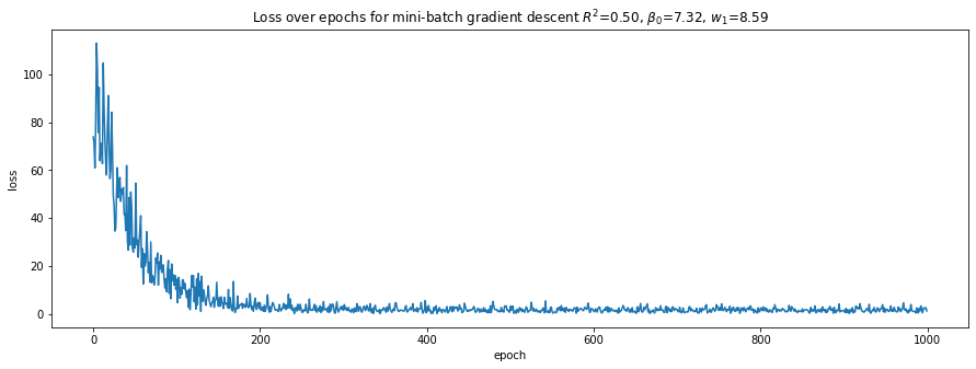
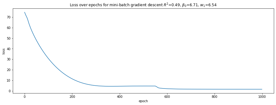
5.2.8. Having fun with 5 layers and mini-batch gradient descent

Here, we define a NN architecture with 5 layers: 1 input, 3 hidden, and 1 output layers. Again, note the mediocre results.

class Net(torch.nn.Module):
    def __init__(self, n_feature, n_hidden, n_output):
        super(Net, self).__init__()
        self.hidden1 = torch.nn.Linear(n_feature, 10, bias=False)
        self.hidden2 = torch.nn.Linear(10, 20, bias=False)
        self.hidden = torch.nn.Linear(20, n_hidden, bias=False)
        self.predict = torch.nn.Linear(n_hidden, n_output, bias=False)

    def forward(self, x):
        x = torch.sigmoid(self.hidden1(x))
        x = torch.sigmoid(self.hidden2(x))
        x = torch.sigmoid(self.hidden(x))
        x = self.predict(x)
        return x

loader = Data.DataLoader(
    dataset=Data.TensorDataset(X, y),
    batch_size=64,
    shuffle=False
)

model = Net(n_feature=2, n_hidden=2, n_output=1)
model = model.to(device)
model.train()

loss_fn = torch.nn.MSELoss(reduction='mean')
learning_rate = 1e-3
optimizer = torch.optim.Adam(model.parameters(), lr=learning_rate)
loss_trace = []

for epoch in range(1000):
    for step, (batch_x, batch_y) in enumerate(loader):
        optimizer.zero_grad()

        with torch.set_grad_enabled(True):
            y_pred = model(batch_x)
            loss = loss_fn(y_pred, batch_y)

            loss.backward()
            optimizer.step()
    loss_trace.append((epoch, loss.item()))

model.eval()
r2 = r2_score(model(X).cpu().detach().numpy(), y.cpu().detach().numpy())
b0 = model.predict.weight[0, 0].cpu().detach().numpy()
w1 = model.predict.weight[0, 1].cpu().detach().numpy()
plot_loss(loss_trace, r'Loss over epochs for mini-batch gradient descent $R^2$={:.2f}, $\beta_0$={:.2f}, $w_1$={:.2f}'.format(r2, b0, w1))