8. K-means, BIC, AIC

8.1. Data

import numpy as np
import random
from numpy.random import normal
from collections import namedtuple

Data = namedtuple('Data', 'X y')

random.seed(37)
np.random.seed(37)

def get_data(means, variances, labels, N=1000):
    def get_X(sample_means, sample_variances, N):
        return np.hstack([normal(m, v, N).reshape(-1, 1) for m, v in zip(sample_means, sample_variances)])

    def get_y(label, N):
        return np.full(N, label, dtype=np.int)

    X = np.vstack([get_X(m, v, N) for m, v in zip(means, variances)])
    y = np.hstack([get_y(label, N) for label in labels])

    return Data(X, y)

# training
means = [
    [5.0, 5.0],
    [99.0, 99.0],
    [15.0, 20.0]
]
variances = [
    [1.0, 1.0],
    [1.0, 1.0],
    [1.0, 1.0]
]
labels = range(len(means))

X, y = get_data(means=means, variances=variances, labels=labels)

print(f'X shape = {X.shape}, y shape {y.shape}')

X shape = (3000, 2), y shape (3000,)

8.2. BIC, AIC and more

from sklearn.cluster import KMeans
from sklearn.metrics import silhouette_score, davies_bouldin_score
from sklearn.metrics import homogeneity_score, completeness_score, v_measure_score
from sklearn.metrics import calinski_harabasz_score
from sklearn.mixture import GaussianMixture
from scipy.stats import multivariate_normal as mvn

def get_km(k, X):
    km = KMeans(n_clusters=k, random_state=37)
    km.fit(X)
    return km

def get_bic_aic(k, X):
    gmm = GaussianMixture(n_components=k, init_params='kmeans')
    gmm.fit(X)
    return gmm.bic(X), gmm.aic(X)

def get_score(k, X, y):
    km = get_km(k, X)
    y_pred = km.predict(X)
    bic, aic = get_bic_aic(k, X)
    sil = silhouette_score(X, y_pred)
    db = davies_bouldin_score(X, y_pred)
    hom = homogeneity_score(y, y_pred)
    com = completeness_score(y, y_pred)
    vms = v_measure_score(y, y_pred)
    cal = calinski_harabasz_score(X, y_pred)
    return k, bic, aic, sil, db, hom, com, vms, cal

The meaning of the scores.

• BIC lower is better

• AIC lower is better

• silhouette higher is better

• davies lower is better

• homogeneity higher is better

• completeness higher is better

• v-measure higher is better

• calinski higher is better

import pandas as pd

df = pd.DataFrame([get_score(k, X, y) for k in range(2, 11)],
                  columns=['k', 'BIC', 'AIC', 'silhouette',
                           'davies', 'homogeneity',
                           'completeness', 'vmeasure', 'calinski'])
df

	k	BIC	AIC	silhouette	davies	homogeneity	completeness	vmeasure	calinski
0	2	29713.687099	29647.617056	0.941677	0.082989	0.57938	1.000000	0.733680	1.827224e+05
1	3	23709.628278	23607.520029	0.929479	0.099672	1.00000	1.000000	1.000000	2.623227e+06
2	4	23764.812594	23626.666140	0.731644	0.660094	1.00000	0.828906	0.906450	1.963947e+06
3	5	23812.883924	23638.699264	0.504188	1.032971	1.00000	0.703982	0.826279	1.672838e+06
4	6	23856.161363	23645.938498	0.306449	1.264110	1.00000	0.613262	0.760275	1.541983e+06
5	7	23898.831307	23652.570237	0.313627	1.128982	1.00000	0.573512	0.728958	1.437240e+06
6	8	23941.542123	23659.242848	0.324070	1.015535	1.00000	0.534216	0.696402	1.407921e+06
7	9	23986.361374	23668.023893	0.329671	0.952718	1.00000	0.502211	0.668629	1.422252e+06
8	10	24035.079248	23680.703562	0.326965	0.955671	1.00000	0.480658	0.649249	1.366897e+06

8.3. Visualize

%matplotlib inline
import matplotlib.pyplot as plt
from sklearn.preprocessing import MinMaxScaler

plt.style.use('ggplot')

def plot_compare(df, y1, y2, x, fig, ax1):
    ax1.plot(df[x], df[y1], color='tab:red')
    ax1.set_title(f'{y1} and {y2}')
    ax1.set_xlabel(x)
    ax1.set_ylabel(y1, color='tab:red')
    ax1.tick_params(axis='y', labelcolor='tab:red')

    ax2 = ax1.twinx()
    ax2.plot(df[x], df[y2], color='tab:blue')
    ax2.set_ylabel(y2, color='tab:blue')
    ax2.tick_params(axis='y', labelcolor='tab:blue')

def plot_contrast(df, y1, y2, x, fig, ax):
    a = np.array(df[y1])
    b = np.array(df[y2])

    r_min, r_max = df[y1].min(), df[y1].max()
    scaler = MinMaxScaler(feature_range=(r_min, r_max))
    b = scaler.fit_transform(b.reshape(-1, 1))[:,0]

    diff = np.abs(a - b)
    ax.plot(df[x], diff)
    ax.set_title('Scaled Absolute Difference')
    ax.set_xlabel(x)
    ax.set_ylabel('absolute difference')

def plot_result(df, y1, y2, x):
    fig, axes = plt.subplots(1, 2, figsize=(10, 3))
    plot_compare(df, y1, y2, x, fig, axes[0])
    plot_contrast(df, y1, y2, x, fig, axes[1])
    plt.tight_layout()

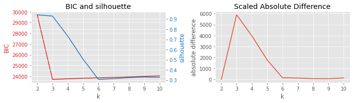
8.3.1. BIC vs silhouette

plot_result(df, 'BIC', 'silhouette', 'k')

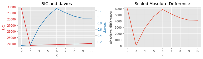
8.3.2. BIC vs Davies-Bouldin

plot_result(df, 'BIC', 'davies', 'k')

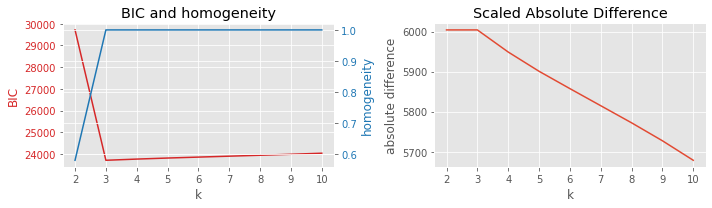
8.3.3. BIC vs homogeneity

plot_result(df, 'BIC', 'homogeneity', 'k')

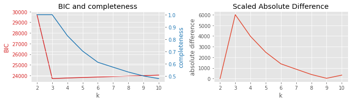
8.3.4. BIC vs completeness

plot_result(df, 'BIC', 'completeness', 'k')

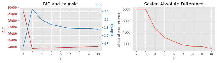
8.3.5. BIC vs Calinski-Harabasz

plot_result(df, 'BIC', 'calinski', 'k')

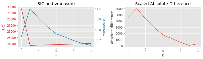
8.3.6. BIC vs v-measure

plot_result(df, 'BIC', 'vmeasure', 'k')