13. Linear Mixed-Effect Regression

Linear Mixed-Effect Regression (LMER) take on the following functional form,

\(y = X \beta + Z u + \epsilon\),

where

• \(y\) is the dependent variable

• \(X\) is the design matrix for fixed effects (variables that have a constant effect on \(y\) regardless of groups),

• \(Z\) is the design matrix for random effects (variables that have different effects on \(y\) across groups),

• \(\beta\) is a vector of the coefficients for the fixed effects corresponding to \(X\),

• \(u\) is a vector of the coefficients for the random effects corresponding to \(Z\), and

• \(\epsilon\) is the random error.

LMER models are typically used to model data that can be grouped. For example, if you have a dataset of elementary students, they can be grouped into classrooms. The data being able to be grouped implies that the units (eg students) are related. Since the units are related, normal regression, like ordinary least-squares (OLS), may be inappropriate when they assume that units are independently and identically distributed (IID). Let’s take a look at LMER modeling.

13.1. Load data

The data and code below is taken from this post and were part of a study in which 30 female rats were randomly assigned to receive one of three doses (High, Low, or Control) of an experimental compound and the weights of their pups were measured as the effect of the chemical compound. The lowest unit of analysis is at the pup level, and these pups are further grouped into litters. We have the following variables.

• \(y\) = weight

• \(X\) = {sex, litsize, treatment}

• \(Z\) = litter

import pandas as pd

df = pd.read_csv('http://www-personal.umich.edu/~bwest/rat_pup.dat', sep='\t') \
    .set_index(['pup_id'])
df.shape

(322, 5)

df.dtypes

weight       float64
sex           object
litter         int64
litsize        int64
treatment     object
dtype: object

df.info()

<class 'pandas.core.frame.DataFrame'>
Int64Index: 322 entries, 1 to 322
Data columns (total 5 columns):
 #   Column     Non-Null Count  Dtype
---  ------     --------------  -----
 0   weight     322 non-null    float64
 1   sex        322 non-null    object
 2   litter     322 non-null    int64
 3   litsize    322 non-null    int64
 4   treatment  322 non-null    object
dtypes: float64(1), int64(2), object(2)
memory usage: 15.1+ KB

df.isna().sum()

weight       0
sex          0
litter       0
litsize      0
treatment    0
dtype: int64

df.head()

	weight	sex	litter	litsize	treatment
pup_id
1	6.60	Male	1	12	Control
2	7.40	Male	1	12	Control
3	7.15	Male	1	12	Control
4	7.24	Male	1	12	Control
5	7.10	Male	1	12	Control

13.2. Visualize features

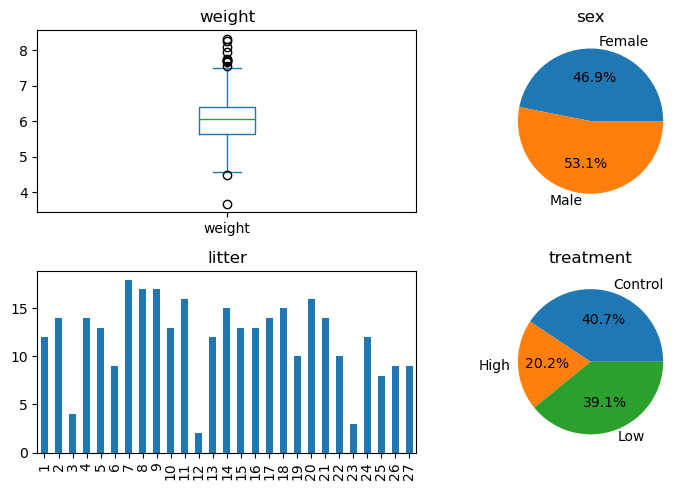
Now let’s pick some visualization to summarize each variable.

• The median weight is 6.

• There are more males (53%) than females (47%).

• There is imbalance across the litters.

• About 41% of the rat pups came from mothers that were not treated, followed by 39% whose mothers were treated with a low dose and 20% whose mothers were treated with a high dose.

import matplotlib.pyplot as plt
import numpy as np

fig, ax = plt.subplots(2, 2, figsize=(8, 5))
ax = np.ravel(ax)

df['weight'].plot(kind='box', ax=ax[0])
df['sex'].value_counts().sort_index().plot(kind='pie', autopct='%1.1f%%', ax=ax[1])
df['litter'].value_counts().sort_index().plot(kind='bar', ax=ax[2])
df['treatment'].value_counts().sort_index().plot(kind='pie', autopct='%1.1f%%', ax=ax[3])

ax[0].set_title('weight')
ax[1].set_title('sex')
ax[2].set_title('litter')
ax[3].set_title('treatment')
ax[1].set_ylabel('')
ax[3].set_ylabel('')

fig.tight_layout()

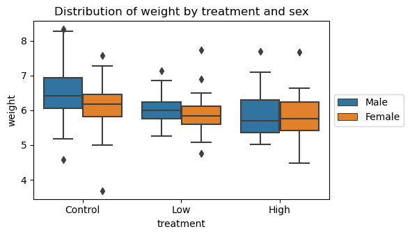
13.3. Visualize weights by treatment and sex

We can see that the median weight for both males and females trend from high to low as we move from the control to low to high-treatment groups.

import seaborn as sns

fig, ax = plt.subplots(figsize=(6, 3.5))

sns.boxplot(data=df, x='treatment', y='weight', hue='sex', ax=ax)

ax.set_title('Distribution of weight by treatment and sex')
ax.legend(loc='center left', bbox_to_anchor=(1, 0.5))

fig.tight_layout()

13.4. Linear model

Let’s use a simple linear model for the data.

\(y = X \beta + \epsilon\)

import statsmodels.formula.api as smf

ols_model = smf.ols(
        formula='''weight ~ litsize + C(treatment) + C(sex, Treatment("Male"))''',
        data=df) \
    .fit()

ols_model.summary()

OLS Regression Results

Dep. Variable:	weight	R-squared:	0.409
Model:	OLS	Adj. R-squared:	0.401
Method:	Least Squares	F-statistic:	54.76
Date:	Fri, 18 Aug 2023	Prob (F-statistic):	4.56e-35
Time:	09:45:07	Log-Likelihood:	-231.84
No. Observations:	322	AIC:	473.7
Df Residuals:	317	BIC:	492.5
Df Model:	4
Covariance Type:	nonrobust

	coef	std err	t	P>|t|	[0.025	0.975]
Intercept	8.2240	0.156	52.864	0.000	7.918	8.530
C(treatment)[T.High]	-0.9062	0.086	-10.554	0.000	-1.075	-0.737
C(treatment)[T.Low]	-0.4250	0.063	-6.754	0.000	-0.549	-0.301
C(sex, Treatment("Male"))[T.Female]	-0.2739	0.056	-4.863	0.000	-0.385	-0.163
litsize	-0.1249	0.010	-12.236	0.000	-0.145	-0.105

Omnibus:	61.833	Durbin-Watson:	1.415
Prob(Omnibus):	0.000	Jarque-Bera (JB):	292.290
Skew:	-0.693	Prob(JB):	3.39e-64
Kurtosis:	7.457	Cond. No.	82.0

Notes:
[1] Standard Errors assume that the covariance matrix of the errors is correctly specified.

13.5. LMER, random intercept model

Now, we will use a LMER model allowing for the intercept to change. What do we mean by “allowing for the intercept to change?” We mean that there will be a different expected mean for each group (in the running example, each group is a litter of rat pups). Note the use of the groups parameter which is set to litter.

rim_model = smf.mixedlm(
        formula='''weight ~ litsize + C(treatment) + C(sex, Treatment('Male'))''',
        data=df,
        groups='litter') \
    .fit()

rim_model.summary()

Model:	MixedLM	Dependent Variable:	weight
No. Observations:	322	Method:	REML
No. Groups:	27	Scale:	0.1628
Min. group size:	2	Log-Likelihood:	-198.4997
Max. group size:	18	Converged:	Yes
Mean group size:	11.9

	Coef.	Std.Err.	z	P>|z|	[0.025	0.975]
Intercept	8.310	0.274	30.355	0.000	7.773	8.846
C(treatment)[T.High]	-0.859	0.182	-4.722	0.000	-1.215	-0.502
C(treatment)[T.Low]	-0.429	0.150	-2.849	0.004	-0.723	-0.134
C(sex, Treatment('Male'))[T.Female]	-0.359	0.048	-7.540	0.000	-0.452	-0.266
litsize	-0.129	0.019	-6.863	0.000	-0.166	-0.092
litter Var	0.097	0.085

13.6. LMER, random slope model, intercept and slopes independent

In this LMER model, we allow for the slope to change. In the LMER model where we allow for the intercept to change, the slopes are all the same and it is just the intercept that changes. Here, the slopes and intercepts changes per group, but the model does not assume interactions between the slopes and intercepts. Note the use of vc_formula parameter with the dictionary.

rsm_model = smf.mixedlm(
        formula='''weight ~ litsize + C(treatment) + C(sex, Treatment('Male'))''',
        data=df,
        groups='litter',
        vc_formula = {'sex' : '0 + C(sex)'}) \
    .fit()

rsm_model.summary()

Model:	MixedLM	Dependent Variable:	weight
No. Observations:	322	Method:	REML
No. Groups:	27	Scale:	0.1565
Min. group size:	2	Log-Likelihood:	-205.7020
Max. group size:	18	Converged:	Yes
Mean group size:	11.9

	Coef.	Std.Err.	z	P>|z|	[0.025	0.975]
Intercept	8.231	0.234	35.185	0.000	7.772	8.689
C(treatment)[T.High]	-0.839	0.144	-5.827	0.000	-1.121	-0.557
C(treatment)[T.Low]	-0.411	0.116	-3.526	0.000	-0.639	-0.182
C(sex, Treatment('Male'))[T.Female]	-0.356	0.102	-3.508	0.000	-0.555	-0.157
litsize	-0.124	0.016	-7.915	0.000	-0.155	-0.093
sex Var	0.104	0.076

13.7. LMER, random slope model, intercept and slopes dependent

In this LMER model, we allow for the slopes and intercepts to change and assume an interaction between the two. Note the use of re_formula and string literal formula.

ris_model = smf.mixedlm(
        formula='''weight ~ litsize + C(treatment) + C(sex, Treatment('Male'))''',
        data=df,
        groups='litter',
        re_formula = '1 + C(sex)') \
    .fit()

ris_model.summary()

Model:	MixedLM	Dependent Variable:	weight
No. Observations:	322	Method:	REML
No. Groups:	27	Scale:	0.1601
Min. group size:	2	Log-Likelihood:	-196.3946
Max. group size:	18	Converged:	Yes
Mean group size:	11.9

	Coef.	Std.Err.	z	P>|z|	[0.025	0.975]
Intercept	8.166	0.265	30.765	0.000	7.645	8.686
C(treatment)[T.High]	-0.778	0.172	-4.523	0.000	-1.116	-0.441
C(treatment)[T.Low]	-0.387	0.137	-2.821	0.005	-0.656	-0.118
C(sex, Treatment('Male'))[T.Female]	-0.359	0.053	-6.783	0.000	-0.463	-0.255
litsize	-0.120	0.018	-6.637	0.000	-0.155	-0.084
litter Var	0.063	0.074
litter x C(sex)[T.Male] Cov	0.028	0.044
C(sex)[T.Male] Var	0.013	0.062

Below is the estimated correlation coefficient between the random intercepts and random slopes. This correlation indicates that the litters with higher weight tend to have males that are of higher weight.

ris_model.params['litter x C(sex)[T.Male] Cov'] / np.sqrt(ris_model.params['litter Var'] * ris_model.params['C(sex)[T.Male] Var'])

0.9878805022022777

13.8. Performance

Let’s look at the non-validated performance measures. The MAE, RMSE, MAPE and \(R^2\) are all comparable between these models, but the log-likelihood is better for the random intercept, random slope model.

• RIS: random intercept, random slope

• RIM: random intercept

• RSM: random slope

• OLS: ordinary least square

from sklearn.metrics import mean_absolute_error, mean_squared_error, mean_absolute_percentage_error, r2_score

def get_performance(m, X, y_true, Z=None, clusters=None):
    if Z is not None and clusters is not None:
        y_pred = m.predict(X, Z, clusters)
    else:
        y_pred  = m.predict(X)

    mae = mean_absolute_error(y_true, y_pred)
    rmse = mean_squared_error(y_true, y_pred, squared=False)
    mape = mean_absolute_percentage_error(y_true, y_pred)
    rsq = r2_score(y_true, y_pred)

    try:
        ll = m.llf
    except:
        ll = np.nan

    y_pred = pd.Series([mae, rmse, mape, rsq, ll], index=['mae', 'rmse', 'mape', 'r-sq', 'log-likelihood'])
    return y_pred

lmer_df = pd.DataFrame([get_performance(m, df[['litsize', 'treatment', 'sex', 'litter']], df['weight'])
              for m in [ols_model, rim_model, rsm_model, ris_model]],
             index=['OLS', 'RIM', 'RSM', 'RIS']) \
    .sort_values(['log-likelihood'], ascending=False)
lmer_df

	mae	rmse	mape	r-sq	log-likelihood
RIS	0.383076	0.500760	0.064635	0.399894	-196.394596
RIM	0.382219	0.499605	0.064361	0.402659	-198.499691
RSM	0.381596	0.499295	0.064256	0.403400	-205.702007
OLS	0.376124	0.497108	0.063282	0.408616	-231.836723

13.9. Mixed-Effects Random Forest

Mixed-Effects Random Forest (MERF) is another approach to mixed-effect modeling. The functional form of the model is as follows,

• \(y_i = f(X_i) + Z_i u_i + e_i\)

• \(u_i \sim \mathcal{N}(0, D)\)

• \(e_i \sim \mathcal{N}(0, \sigma_i)\)

where,

• \(y_i\) is the vector of responses for the i-th cluster,

• \(X_i\) is the fixed effects covariates associated with \(y_i\),

• \(Z_i\) is the random effects covariates associated with the \(y_i\), and

• \(e_i \sim \mathcal{N}(0, \sigma_i)\) is the vector of error for the i-th cluster.

The learned parameters in MERF are

• \(f()\): a random forest that models the (potentially nonlinear) mapping from the fixed effect covariates to the response (common across all clusters),

• \(D\): the covariance of the normal distribution from which each \(u_i\) is drawn, and

• \(\sigma_i\): the variance of \(e_i\).

The random effects, \(Z_i u_i\), is still assumed to be linear.

To use MERF, install the following package.

pip install git+https://github.com/manifoldai/merf.git

Now let’s shape the data for input into MERF.

sex_map = {'Male': 1, 'Female': 0}
treatment_map = {'Control': 0, 'Low': 1, 'High': 2}

X = df[['litsize', 'treatment', 'sex']] \
        .assign(
            sex=lambda d: d['sex'].map(sex_map),
            treatment=lambda d: d['treatment'].map(treatment_map)
        )
# Z = pd.DataFrame({'Z': np.ones(X.shape[0])}, index=X.index)
Z = df[['sex']].assign(sex=lambda d: d['sex'].map(sex_map))
clusters = df['litter']
y = df['weight']

X.shape, Z.shape, y.shape, clusters.shape

((322, 3), (322, 1), (322,), (322,))

By default, MERF uses a random forest to model the fixed effects. You will see that the way the parameters are learned is through an iteration procedure. In particular, the parameters are learned using the Expectation-Maximization Algorithm.

from merf import MERF
from sklearn.ensemble import RandomForestRegressor

merf = MERF(
    fixed_effects_model=RandomForestRegressor(n_estimators=30, n_jobs=-1, random_state=37),
    max_iterations=20
)
merf.fit(X, Z, clusters, y)

INFO     [merf.py:307] Training GLL is -333.71605873307544 at iteration 1.
INFO     [merf.py:307] Training GLL is -377.01192150920764 at iteration 2.
INFO     [merf.py:307] Training GLL is -385.0144049452151 at iteration 3.
INFO     [merf.py:307] Training GLL is -388.49413213816604 at iteration 4.
INFO     [merf.py:307] Training GLL is -390.786958923229 at iteration 5.
INFO     [merf.py:307] Training GLL is -392.6172680813943 at iteration 6.
INFO     [merf.py:307] Training GLL is -394.1013482379355 at iteration 7.
INFO     [merf.py:307] Training GLL is -395.3064926013952 at iteration 8.
INFO     [merf.py:307] Training GLL is -396.2790567471805 at iteration 9.
INFO     [merf.py:307] Training GLL is -397.0650753333675 at iteration 10.
INFO     [merf.py:307] Training GLL is -397.70311641522136 at iteration 11.
INFO     [merf.py:307] Training GLL is -398.2237484173181 at iteration 12.
INFO     [merf.py:307] Training GLL is -398.65074861675413 at iteration 13.
INFO     [merf.py:307] Training GLL is -399.00256401978334 at iteration 14.
INFO     [merf.py:307] Training GLL is -399.29357896736184 at iteration 15.
INFO     [merf.py:307] Training GLL is -399.5351033681913 at iteration 16.
INFO     [merf.py:307] Training GLL is -399.7361114952454 at iteration 17.
INFO     [merf.py:307] Training GLL is -399.90378716325665 at iteration 18.
INFO     [merf.py:307] Training GLL is -400.0439266668877 at iteration 19.
INFO     [merf.py:307] Training GLL is -400.16123920919347 at iteration 20.

<merf.merf.MERF at 0x7f8f9830d850>

You can see from the merged results of LMER and MERF that MERF performs better (non-validated).

merf_df = pd.DataFrame([get_performance(merf, X, y, Z, clusters)], index=['MERF'])

pd.concat([lmer_df, merf_df])

	mae	rmse	mape	r-sq	log-likelihood
RIS	0.383076	0.500760	0.064635	0.399894	-196.394596
RIM	0.382219	0.499605	0.064361	0.402659	-198.499691
RSM	0.381596	0.499295	0.064256	0.403400	-205.702007
OLS	0.376124	0.497108	0.063282	0.408616	-231.836723
MERF	0.278688	0.376164	0.046600	0.661372	NaN

MERF is flexible enough to allow any linear or non-linear regressor to model the fixed effects. We are using a linear model here to model the fixed effects. This linear model for the fixed effects using the MERF API should reduce back to LMER.

from sklearn.linear_model import LinearRegression

merf_linear = MERF(
    fixed_effects_model=LinearRegression(),
    max_iterations=20
)
merf_linear.fit(X, Z, clusters, y)

INFO     [merf.py:307] Training GLL is -250.32226566191966 at iteration 1.
INFO     [merf.py:307] Training GLL is -275.4248038416475 at iteration 2.
INFO     [merf.py:307] Training GLL is -278.405863266045 at iteration 3.
INFO     [merf.py:307] Training GLL is -279.14089177633406 at iteration 4.
INFO     [merf.py:307] Training GLL is -279.39470078845005 at iteration 5.
INFO     [merf.py:307] Training GLL is -279.50761907216946 at iteration 6.
INFO     [merf.py:307] Training GLL is -279.56454572394097 at iteration 7.
INFO     [merf.py:307] Training GLL is -279.59504914913975 at iteration 8.
INFO     [merf.py:307] Training GLL is -279.6118859892217 at iteration 9.
INFO     [merf.py:307] Training GLL is -279.62124285234916 at iteration 10.
INFO     [merf.py:307] Training GLL is -279.6263549945002 at iteration 11.
INFO     [merf.py:307] Training GLL is -279.62900945894233 at iteration 12.
INFO     [merf.py:307] Training GLL is -279.6302331119333 at iteration 13.
INFO     [merf.py:307] Training GLL is -279.63063176871344 at iteration 14.
INFO     [merf.py:307] Training GLL is -279.6305682053091 at iteration 15.
INFO     [merf.py:307] Training GLL is -279.63026066897373 at iteration 16.
INFO     [merf.py:307] Training GLL is -279.62983973763113 at iteration 17.
INFO     [merf.py:307] Training GLL is -279.62938219900144 at iteration 18.
INFO     [merf.py:307] Training GLL is -279.62893170266136 at iteration 19.
INFO     [merf.py:307] Training GLL is -279.6285115436138 at iteration 20.

<merf.merf.MERF at 0x7f8fbc55deb0>

In this MERF example, we use something fancier, gradient boosting, to model the fixed effects.

from lightgbm import LGBMRegressor

merf_lbgm = MERF(
    fixed_effects_model=LGBMRegressor(),
    max_iterations=20
)
merf_lbgm.fit(X, Z, clusters, y)

INFO     [merf.py:307] Training GLL is -280.8403423506038 at iteration 1.
INFO     [merf.py:307] Training GLL is -312.5902759696268 at iteration 2.
INFO     [merf.py:307] Training GLL is -319.42122808679375 at iteration 3.
INFO     [merf.py:307] Training GLL is -323.30449745760814 at iteration 4.
INFO     [merf.py:307] Training GLL is -325.39602517001947 at iteration 5.
INFO     [merf.py:307] Training GLL is -325.97589056606364 at iteration 6.
INFO     [merf.py:307] Training GLL is -326.50014975589113 at iteration 7.
INFO     [merf.py:307] Training GLL is -326.6869382890954 at iteration 8.
INFO     [merf.py:307] Training GLL is -326.67740437411493 at iteration 9.
INFO     [merf.py:307] Training GLL is -326.7714395331036 at iteration 10.
INFO     [merf.py:307] Training GLL is -327.54464523883496 at iteration 11.
INFO     [merf.py:307] Training GLL is -327.09840142944836 at iteration 12.
INFO     [merf.py:307] Training GLL is -327.4145901178239 at iteration 13.
INFO     [merf.py:307] Training GLL is -327.5149945679775 at iteration 14.
INFO     [merf.py:307] Training GLL is -327.76484590606526 at iteration 15.
INFO     [merf.py:307] Training GLL is -326.04470343017886 at iteration 16.
INFO     [merf.py:307] Training GLL is -327.4639939165594 at iteration 17.
INFO     [merf.py:307] Training GLL is -327.7250271749926 at iteration 18.
INFO     [merf.py:307] Training GLL is -326.68773048443546 at iteration 19.
INFO     [merf.py:307] Training GLL is -326.8288576814248 at iteration 20.

<merf.merf.MERF at 0x7f8fbc54d370>

The table below compares the LMER and MERF models. In general, MERF models using a non-linear model for the fixed effects does better than LMER models across all (non-validated) performance measures. The problem with random forest and gradient boosting is they have a higher chance to overfit as they have higher variance, as opposed to the LMER models, which have higher bias (see bias-variance tradeoff).

linear_df = pd.DataFrame([get_performance(merf_linear, X, y, Z, clusters)], index=['MERF_LINEAR'])
lgbm_df = pd.DataFrame([get_performance(merf_lbgm, X, y, Z, clusters)], index=['MERF_LGBM'])

pd.concat([lmer_df, merf_df, linear_df, lgbm_df])

	mae	rmse	mape	r-sq	log-likelihood
RIS	0.383076	0.500760	0.064635	0.399894	-196.394596
RIM	0.382219	0.499605	0.064361	0.402659	-198.499691
RSM	0.381596	0.499295	0.064256	0.403400	-205.702007
OLS	0.376124	0.497108	0.063282	0.408616	-231.836723
MERF	0.278688	0.376164	0.046600	0.661372	NaN
MERF_LINEAR	0.303176	0.415935	0.051168	0.585982	NaN
MERF_LGBM	0.286231	0.405772	0.047979	0.605967	NaN

13.10. Learned parameters

Since model interpretability is important, you should look at the learned parameters. These are the parameters for the LMER model with random slopes and intercepts (slopes and intercepts are dependent).

ris_model.params

Intercept                              8.165656
C(treatment)[T.High]                  -0.778370
C(treatment)[T.Low]                   -0.387161
C(sex, Treatment('Male'))[T.Female]   -0.359242
litsize                               -0.119568
litter Var                             0.395468
litter x C(sex)[T.Male] Cov            0.175758
C(sex)[T.Male] Var                     0.080040
dtype: float64

For the MERF model using random forest to model the fixed effects, these are the feature importances of the fixed effects. You simply reference the random forest model and the feature_importances_ attribute. Litter size is apparently the most important feature for the fixed effects.

pd.Series(merf.fe_model.feature_importances_, X.columns)

litsize      0.558371
treatment    0.331581
sex          0.110048
dtype: float64

To look at the influence at the group level (litter), print out the trained_b. The nomenclature for MERF is to use \(b\) for the random effect coefficients (as opposed to LMER, which uses \(u\) for the random effect coefficients and \(b\) for the fixed effect coefficients). Do not let this cognitive friction confuse you.

merf.trained_b.sort_index()

	0
1	-0.013010
2	-0.003138
3	0.000726
4	0.002064
5	0.077942
6	-0.002509
7	-0.039926
8	0.211264
9	-0.186452
10	-0.147620
11	-0.112385
12	0.000000
13	-0.025229
14	-0.234172
15	0.006974
16	-0.011536
17	-0.010374
18	0.171552
19	0.023750
20	0.109437
21	0.029966
22	0.045427
23	0.045619
24	0.008777
25	0.077531
26	0.053139
27	-0.108956

13.11. Validation

Let’s split the data 70% (training) and 30% (testing) stratified by the litter identifier.

from sklearn.model_selection import train_test_split

X_tr, X_te, y_tr, y_te = train_test_split(
    df[['litsize', 'treatment', 'sex', 'litter']] \
        .assign(
            sex=lambda d: d['sex'].map(sex_map),
            treatment=lambda d: d['treatment'].map(treatment_map)),
    df['weight'],
    test_size=0.30,
    random_state=37,
    shuffle=True,
    stratify=df['litter']
)

Z_tr = X_tr[['sex']]
Z_te = X_te[['sex']]

C_tr = X_tr['litter']
C_te = X_te['litter']

X_tr = X_tr.drop(columns=['litter'])
X_te = X_te.drop(columns=['litter'])

X_tr.shape, Z_tr.shape, C_tr.shape, y_tr.shape

((225, 3), (225, 1), (225,), (225,))

X_te.shape, Z_te.shape, C_te.shape, y_te.shape

((97, 3), (97, 1), (97,), (97,))

Let’s make sure the proportions of litters in the training and testing folds are preserved.

s1 = df['litter'].value_counts().sort_index()
s2 = C_tr.value_counts().sort_index()
s3 = C_te.value_counts().sort_index()

p1 = s1 / s1.sum()
p2 = s2 / s2.sum()
p3 = s3 / s3.sum()

pd.DataFrame([p1, p2, p3], index=['X', 'X_tr', 'X_te']).T

	X	X_tr	X_te
1	0.037267	0.035556	0.041237
2	0.043478	0.044444	0.041237
3	0.012422	0.013333	0.010309
4	0.043478	0.044444	0.041237
5	0.040373	0.040000	0.041237
6	0.027950	0.026667	0.030928
7	0.055901	0.057778	0.051546
8	0.052795	0.053333	0.051546
9	0.052795	0.053333	0.051546
10	0.040373	0.040000	0.041237
11	0.049689	0.048889	0.051546
12	0.006211	0.004444	0.010309
13	0.037267	0.035556	0.041237
14	0.046584	0.048889	0.041237
15	0.040373	0.040000	0.041237
16	0.040373	0.040000	0.041237
17	0.043478	0.044444	0.041237
18	0.046584	0.048889	0.041237
19	0.031056	0.031111	0.030928
20	0.049689	0.048889	0.051546
21	0.043478	0.044444	0.041237
22	0.031056	0.031111	0.030928
23	0.009317	0.008889	0.010309
24	0.037267	0.035556	0.041237
25	0.024845	0.026667	0.020619
26	0.027950	0.026667	0.030928
27	0.027950	0.026667	0.030928

Now let’s validate.

def get_model():
    model = MERF(
        fixed_effects_model=RandomForestRegressor(n_estimators=30, n_jobs=-1, random_state=37),
        max_iterations=20
    )
    return model

def learn(X_tr, Z_tr, C_tr, y_tr):
    model = get_model()
    model.fit(X_tr, Z_tr, C_tr, y_tr)

    return model

def get_results(X_tr, Z_tr, C_tr, y_tr, X_te, Z_te, C_te, y_te):
    model = learn(X_tr, Z_tr, C_tr, y_tr)

    perf_tr = get_performance(model, X_tr, y_tr, Z_tr, C_tr)
    perf_te = get_performance(model, X_te, y_te, Z_te, C_te)

    return pd.DataFrame([perf_tr, perf_te], index=['tr', 'te']).drop(columns=['log-likelihood']).T

get_results(X_tr, Z_tr, C_tr, y_tr, X_te, Z_te, C_te, y_te)

INFO     [merf.py:307] Training GLL is -241.69649293327376 at iteration 1.
INFO     [merf.py:307] Training GLL is -286.11740133632026 at iteration 2.
INFO     [merf.py:307] Training GLL is -295.49781890130924 at iteration 3.
INFO     [merf.py:307] Training GLL is -300.5394268800354 at iteration 4.
INFO     [merf.py:307] Training GLL is -303.881513426677 at iteration 5.
INFO     [merf.py:307] Training GLL is -306.11984582945183 at iteration 6.
INFO     [merf.py:307] Training GLL is -307.9731073008684 at iteration 7.
INFO     [merf.py:307] Training GLL is -309.2839553256728 at iteration 8.
INFO     [merf.py:307] Training GLL is -310.34791724450554 at iteration 9.
INFO     [merf.py:307] Training GLL is -311.1151258488934 at iteration 10.
INFO     [merf.py:307] Training GLL is -311.7811932910758 at iteration 11.
INFO     [merf.py:307] Training GLL is -312.2844557199853 at iteration 12.
INFO     [merf.py:307] Training GLL is -312.67471304477255 at iteration 13.
INFO     [merf.py:307] Training GLL is -312.93907731918256 at iteration 14.
INFO     [merf.py:307] Training GLL is -313.26082011051926 at iteration 15.
INFO     [merf.py:307] Training GLL is -313.4822415902106 at iteration 16.
INFO     [merf.py:307] Training GLL is -313.66794283765677 at iteration 17.
INFO     [merf.py:307] Training GLL is -313.8245804708934 at iteration 18.
INFO     [merf.py:307] Training GLL is -313.95708548909306 at iteration 19.
INFO     [merf.py:307] Training GLL is -314.11774594780064 at iteration 20.

	tr	te
mae	0.265837	0.328698
rmse	0.366546	0.426194
mape	0.044403	0.054894
r-sq	0.681957	0.553932

The validated MERF performance is still pretty good.