1. Missing Data

In this noteboook, we show how to deal with missing data. We will generate two synthetic datasets and then randomly knockout some of their values to be missing. The first dataset will have its parameters manually specified, while the second dataset will have its parameters randomly generated.

1.1. Manually created example

1.1.1. Synthetic data

In this section we manually generate a dataset while manually specifying the parameters. The number of variables that we are generating is 3, and their means are \([10, 20, 30]\) and the covariance matrix between them is as follows.

\(\left[ {\begin{array}{ccccc} 1, 0, 0\\ 0, 1, 0\\ 0, 0, 1\\ \end{array} } \right]\)

The full data is data.

%matplotlib inline
import numpy as np

np.random.seed(37)

means = np.array([10.0, 20.0, 30.0], dtype=np.float64)
cov = np.array([[1.0, 0.0, 0.0], [0.0, 1.0, 0.0], [0.0, 0.0, 1.0]], dtype=np.float64)
data = np.random.multivariate_normal(means, cov, 100)

Now we randomly generate pairs of indices (row and column) for which we will make the corresponding element missing.

def get_null_indices(num_rows, num_cols, num_nulls=50):
    null_indices = []

    indices_pairs = set()
    while len(null_indices) < num_nulls:
        r = np.random.randint(num_rows)
        c = np.random.randint(num_cols)
        key = '{}-{}'.format(r, c)
        if key not in indices_pairs:
            indices_pairs.add(key)
            t = (r, c)
            null_indices.append(t)

    return null_indices

null_indices = get_null_indices(data.shape[0], data.shape[1])

Let’s create the missing data m_data.

def knockout_data(data, null_indices):
    m_data = np.copy(data)
    for pair in null_indices:
        r = pair[0]
        c = pair[1]
        m_data[r][c] = None
    return m_data

m_data = knockout_data(data, null_indices)

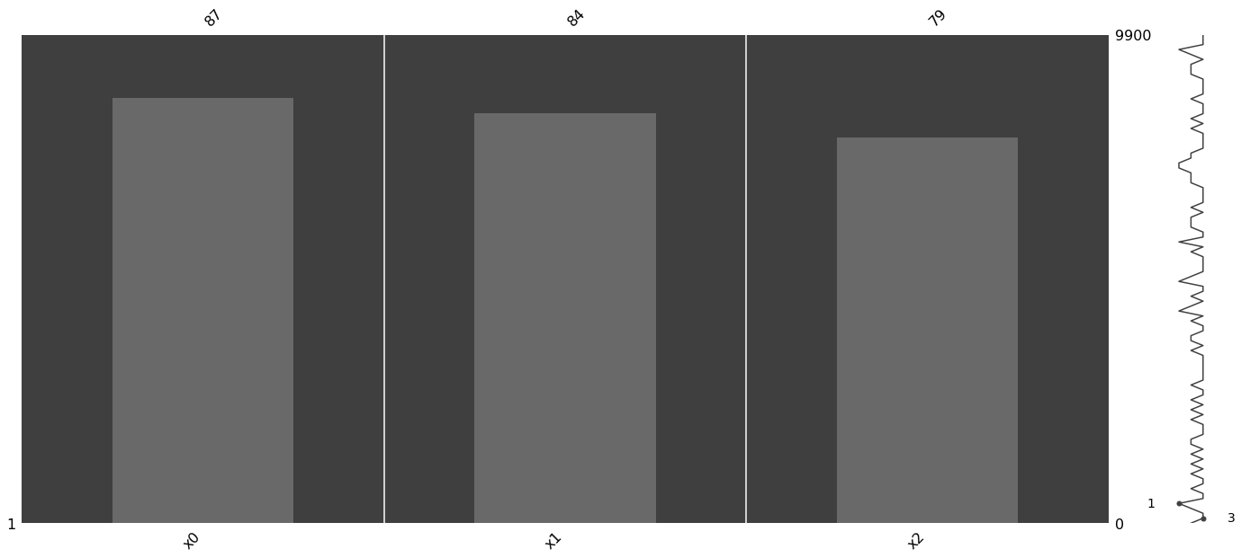
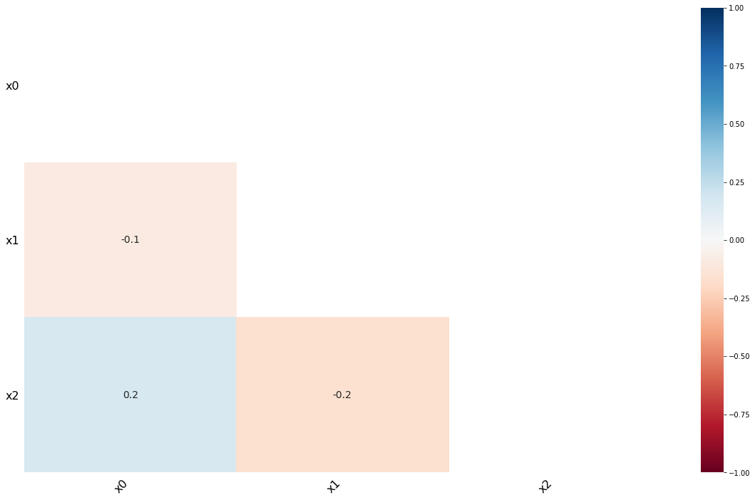
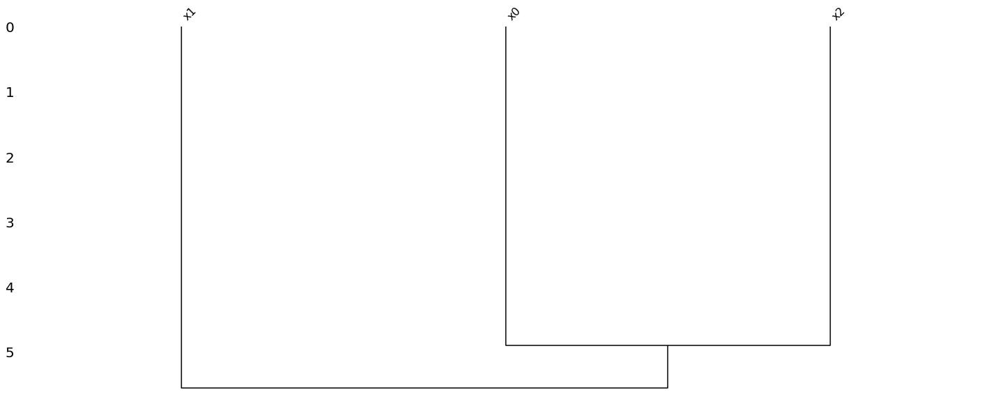
1.1.2. Visualize

import missingno as msno
import matplotlib
import pandas as pd

data_df = pd.DataFrame(m_data, columns=['x{}'.format(c) for c in range(data.shape[1])])

msno.matrix(data_df)
msno.bar(data_df)
msno.heatmap(data_df)
_ = msno.dendrogram(data_df)

1.1.3. Imputation

Let’s impute the missing data using several different techniques.

import warnings
from fancyimpute import KNN
from fancyimpute import NuclearNormMinimization
from fancyimpute import SoftImpute
from fancyimpute import IterativeImputer
from fancyimpute import BiScaler

with warnings.catch_warnings(record=True):
    ii_data = IterativeImputer(verbose=0).fit_transform(m_data)
    nn_data = KNN(k=7, verbose=False).fit_transform(m_data)
    bs_data = BiScaler(verbose=False).fit_transform(m_data)
    si_data = SoftImpute(verbose=False).fit_transform(bs_data)

Using TensorFlow backend.

1.1.4. Performance

Let’s observe the performances of the imputation techniques.

def get_mse(f_data, i_data, null_indices):
    t = []
    for pair in null_indices:
        r, c = pair[0], pair[1]
        v1 = f_data[r][c]
        v2 = i_data[r][c]
        diff = np.power(v1 - v2, 2.0)
        # print('{:.10f}, {:.10f}, {:.10f}'.format(v1, v2, diff))
        t.append(diff)
    t = np.array(t)
    m = np.mean(t)
    return m

def get_mean_mse(f_data, i_data):
    m1 = np.mean(f_data, axis=0)
    m2 = np.mean(i_data, axis=0)
    num_means = len(m1)
    t = []
    for i in range(num_means):
        v1 = m1[i]
        v2 = m2[i]
        diff = np.power(v1 - v2, 2.0)
        t.append(diff)
    t = np.array(t)
    m = np.mean(t)
    return m

def get_cov_mse(f_data, i_data):
    cov1 = np.cov(f_data.T)
    cov2 = np.cov(i_data.T)
    num_rows, num_cols = cov1.shape[0], cov1.shape[1]
    t = []
    for r in range(num_rows):
        for c in range(num_cols):
            v1 = cov1[r][c]
            v2 = cov2[r][c]
            diff = np.power(v1 - v2, 2.0)
            t.append(diff)
    t = np.array(t)
    m = np.mean(t)
    return m

from sklearn.preprocessing import StandardScaler
import pandas as pd

scaler = StandardScaler()
s_data = scaler.fit_transform(data)

perfs = pd.DataFrame([(get_mse(data, ii_data, null_indices),
          get_mean_mse(data, ii_data),
          get_cov_mse(data, ii_data)),
         (get_mse(data, nn_data, null_indices),
          get_mean_mse(data, nn_data),
          get_cov_mse(data, nn_data)),
         (get_mse(s_data, si_data, null_indices),
          get_mean_mse(s_data, si_data),
          get_cov_mse(s_data, si_data))],
        columns=['MSE', 'Average MSE', 'Covariance MSE'],
        index=['Iterative Imputer', 'KNN Imputer', 'Soft Imputer'])

perfs

	MSE	Average MSE	Covariance MSE
Iterative Imputer	0.886978	0.003315	0.008129
KNN Imputer	1.338415	0.003687	0.005270
Soft Imputer	0.988587	0.000258	0.115665

1.2. Randomly generated example

1.2.1. Synthetic data

Now we generate a dataset of 10 random variables with the parameters (means and covariance matrix) generated randomly (as opposed to manually specified as before). We go through the whole process of

• parameter generation,

• data generation,

• missing data creation, and

• imputation.

We then visualize the missingness, followed by computing the performances of the imputation techniques.

num_vars = 10

means = np.array([np.random.randint(20, 100) for i in range(num_vars)], dtype=np.float64)
cov = []
for i in range(num_vars):
    for j in range(num_vars):
        if i == j:
            cov.append(1.0)
        else:
            cov.append(np.random.randint(1, 10))

with warnings.catch_warnings(record=True):
    cov = np.array(cov, dtype=np.float64).reshape((num_vars, num_vars))
    data = np.random.multivariate_normal(means, cov, 500)

    null_indices = get_null_indices(data.shape[0], data.shape[1], num_nulls=1000)
    m_data = knockout_data(data, null_indices)

1.2.2. Imputation

with warnings.catch_warnings(record=True):
    ii_data = IterativeImputer(verbose=0).fit_transform(m_data)
    nn_data = KNN(k=7, verbose=False).fit_transform(m_data)
    bs_data = BiScaler(verbose=False).fit_transform(m_data)
    si_data = SoftImpute(verbose=False).fit_transform(bs_data)

    scaler = StandardScaler()
    s_data = scaler.fit_transform(data)

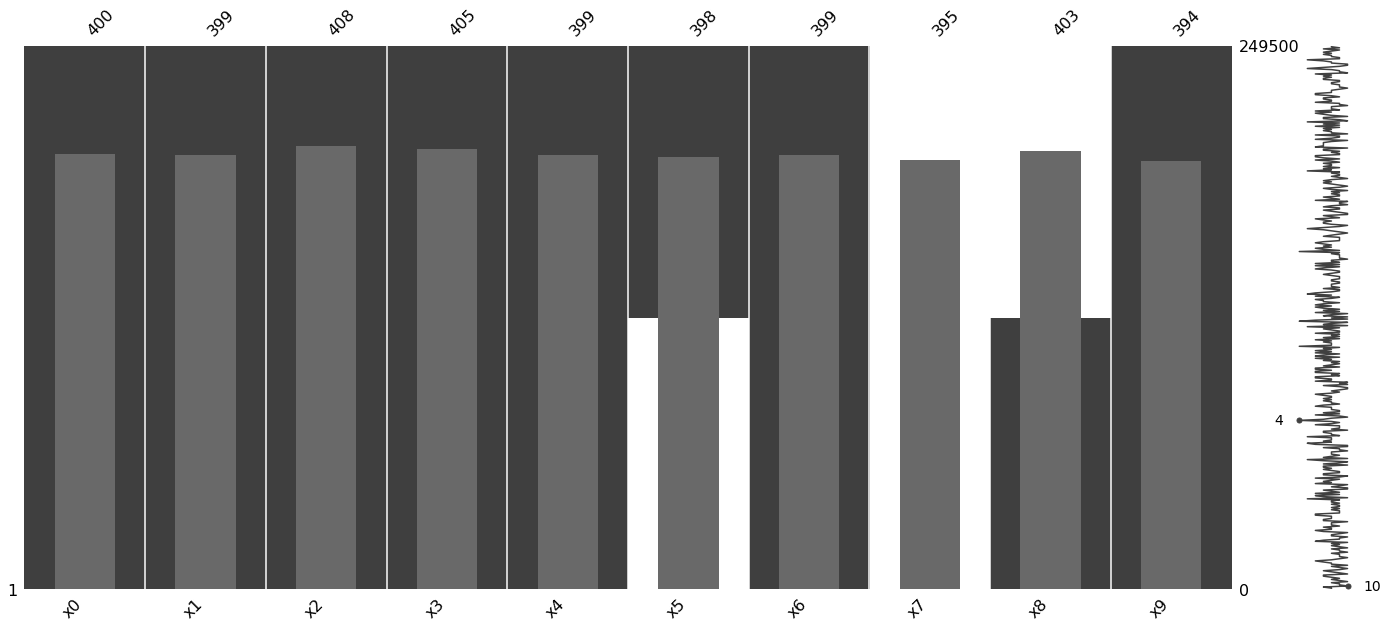
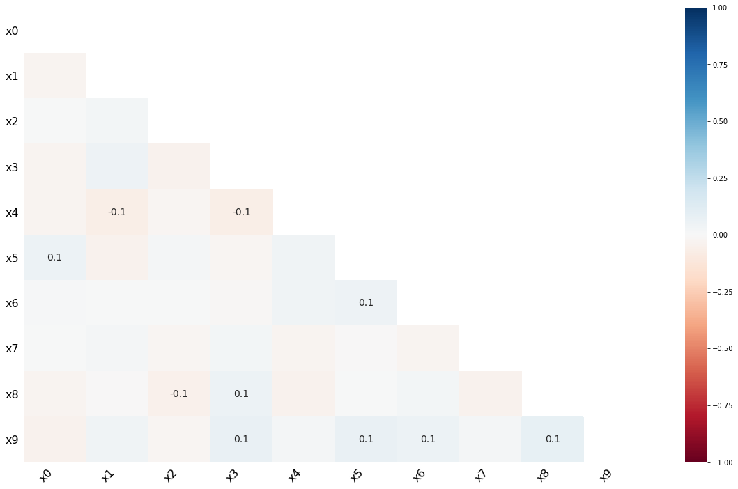
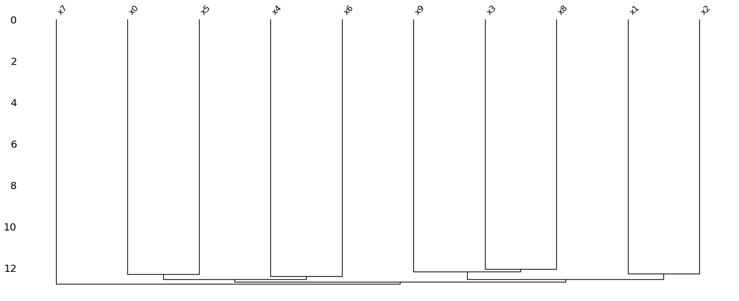
1.2.3. Visualize

data_df = pd.DataFrame(m_data, columns=['x{}'.format(c) for c in range(data.shape[1])])
msno.matrix(data_df)
msno.bar(data_df)
msno.heatmap(data_df)
_ = msno.dendrogram(data_df)

1.2.4. Performance

As can be seen below, iterative imputation seems to do the best by perserving the mean of each variable and also the covariance.

scaler = StandardScaler()
s_data = scaler.fit_transform(data)

perfs = pd.DataFrame([(get_mse(data, ii_data, null_indices),
          get_mean_mse(data, ii_data),
          get_cov_mse(data, ii_data)),
         (get_mse(data, nn_data, null_indices),
          get_mean_mse(data, nn_data),
          get_cov_mse(data, nn_data)),
         (get_mse(s_data, si_data, null_indices),
          get_mean_mse(s_data, si_data),
          get_cov_mse(s_data, si_data))],
        columns=['MSE', 'Average MSE', 'Covariance MSE'],
        index=['Iterative Imputer', 'KNN Imputer', 'Soft Imputer'])

perfs

	MSE	Average MSE	Covariance MSE
Iterative Imputer	6.554412	0.001915	0.141364
KNN Imputer	8.686041	0.007308	0.623918
Soft Imputer	0.909642	0.000009	0.184934