12. Partial Correlation
The purpose of this notebook is to understand how to compute the partial correlation between two variables, \(X\) and \(Y\), given a third \(Z\). In particular, these variables are assumed to be guassians (or, in general, multivariate gaussians).
Why is it important to estimate partial correlations? The primary reason for estimating a partial correlation is to use it to detect for confounding variables during causal analysis.
12.1. Simulation
Let’s start out by simulating 3 data sets. Graphically, these data sets comes from graphs represented by the following.
\(X \rightarrow Z \rightarrow Y\) (serial)
\(X \leftarrow Z \rightarrow Y\) (diverging)
\(X \rightarrow Z \leftarrow Y\) (converging)
[1]:
%matplotlib inline
import matplotlib.pyplot as plt
import networkx as nx
import warnings

warnings.filterwarnings('ignore')
plt.style.use('ggplot')

def get_serial_graph():
    g = nx.DiGraph()

    g.add_node('X')
    g.add_node('Y')
    g.add_node('Z')

    g.add_edge('X', 'Z')
    g.add_edge('Z', 'Y')

    return g

def get_diverging_graph():
    g = nx.DiGraph()

    g.add_node('X')
    g.add_node('Y')
    g.add_node('Z')

    g.add_edge('Z', 'X')
    g.add_edge('Z', 'Y')

    return g

def get_converging_graph():
    g = nx.DiGraph()

    g.add_node('X')
    g.add_node('Y')
    g.add_node('Z')

    g.add_edge('X', 'Z')
    g.add_edge('Y', 'Z')

    return g

g_serial = get_serial_graph()
g_diverging = get_diverging_graph()
g_converging = get_converging_graph()

p_serial = nx.nx_agraph.graphviz_layout(g_serial, prog='dot', args='-Kcirco')
p_diverging = nx.nx_agraph.graphviz_layout(g_diverging, prog='dot', args='-Kcirco')
p_converging = nx.nx_agraph.graphviz_layout(g_converging, prog='dot', args='-Kcirco')

fig, ax = plt.subplots(3, 1, figsize=(5, 5))

nx.draw(g_serial, pos=p_serial, with_labels=True, node_color='#e0e0e0', node_size=800, arrowsize=20, ax=ax[0])
nx.draw(g_diverging, pos=p_diverging, with_labels=True, node_color='#e0e0e0', node_size=800, arrowsize=20, ax=ax[1])
nx.draw(g_converging, pos=p_converging, with_labels=True, node_color='#e0e0e0', node_size=800, arrowsize=20, ax=ax[2])

ax[0].set_title('Serial')
ax[1].set_title('Diverging')
ax[2].set_title('Converging')

plt.tight_layout()
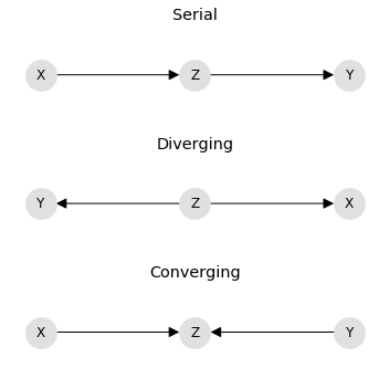
In the serial graph, X causes Z and Z causes Y. In the diverging graph, Z causes both X and Y. In the converging graph, X and Y cause Z. Below, the serial, diverging, and converging data sets are named S, D, and C, correspondingly.
Note that in the serial graph, the data is sampled as follows.
\(X \sim \mathcal{N}(0, 1)\)
\(Z \sim 2 + 1.8 \times X\)
\(Y \sim 5 + 2.7 \times Z\)
In the diverging graph, the data is sampled as follows.
\(Z \sim \mathcal{N}(0, 1)\)
\(X \sim 4.3 + 3.3 \times Z\)
\(Y \sim 5.0 + 2.7 \times Z\)
Lastly, in the converging graph, the data is sampled as follows.
\(X \sim \mathcal{N}(0, 1)\)
\(Y \sim \mathcal{N}(5.5, 1)\)
\(Z \sim 2.0 + 0.8 \times X + 1.2 \times Y\)
Note the ordering of the sampling with the variables follows the structure of the corresponding graph.
[2]:
import numpy as np

np.random.seed(37)

def get_error(N=10000, mu=0.0, std=0.2):
    return np.random.normal(mu, std, N)

def to_matrix(X, Z, Y):
    return np.concatenate([
        X.reshape(-1, 1),
        Z.reshape(-1, 1),
        Y.reshape(-1, 1)], axis=1)

def get_serial(N=10000, e_mu=0.0, e_std=0.2):
    X = np.random.normal(0, 1, N) + get_error(N, e_mu, e_std)
    Z = 2 + 1.8 * X + get_error(N, e_mu, e_std)
    Y = 5 + 2.7 * Z + get_error(N, e_mu, e_std)

    return to_matrix(X, Z, Y)

def get_diverging(N=10000, e_mu=0.0, e_std=0.2):
    Z = np.random.normal(0, 1, N) + get_error(N, e_mu, e_std)
    X = 4.3 + 3.3 * Z + get_error(N, e_mu, e_std)
    Y = 5 + 2.7 * Z + get_error(N, e_mu, e_std)

    return to_matrix(X, Z, Y)

def get_converging(N=10000, e_mu=0.0, e_std=0.2):
    X = np.random.normal(0, 1, N) + get_error(N, e_mu, e_std)
    Y = np.random.normal(5.5, 1, N) + get_error(N, e_mu, e_std)
    Z = 2 + 0.8 * X + 1.2 * Y + get_error(N, e_mu, e_std)

    return to_matrix(X, Z, Y)
[3]:
S = get_serial()
D = get_diverging()
C = get_converging()
12.2. Computation
For the three datasets, S, D, and C, we want to compute the partial correlation between \(X\) and \(Y\) given \(Z\). The way to do this is as follows.
Regress \(X\) on \(Z\) and also \(Y\) on \(Z\)
\(X = b_X + w_X * Z\)
\(Y = b_Y + w_Y * Z\)
With the new weights \((b_X, w_X)\) and \((b_Y, w_Y)\), predict \(X\) and \(Y\).
\(\hat{X} = b_X + w_X * Z\)
\(\hat{Y} = b_Y + w_Y * Z\)
Now compute the residuals between the true and predicted values.
\(R_X = X - \hat{X}\)
\(R_Y = Y - \hat{Y}\)
Finally, compute the Pearson correlation between \(R_X\) and \(R_Y\).
The correlation between the residuals is the partial correlation and runs from -1 to +1. More interesting is the test of significance. If \(p > \alpha\), where \(\alpha \in [0.1, 0.05, 0.01]\), then assume independence. For example, assume \(\alpha = 0.01\) and \(p = 0.002\), then \(X\) is conditionally independent of \(Y\) given \(Z\).
[4]:
from sklearn.linear_model import LinearRegression
from sklearn.metrics import r2_score
from scipy.stats import pearsonr
from scipy import stats

def get_cond_indep_test(c_xy_z, N=10000, alpha=0.01):
    point = stats.norm.ppf(1 - (alpha / 2.0))
    z_transform = np.sqrt(N - 3) * np.abs(0.5 * np.log((1 + c_xy_z) / (1 - c_xy_z)))
    return z_transform, point, z_transform > point

def get_partial_corr(M):
    X = M[:, 0]
    Z = M[:, 1].reshape(-1, 1)
    Y = M[:, 2]

    mXZ = LinearRegression()
    mXZ.fit(Z, X)
    pXZ = mXZ.predict(Z)
    rXZ = X - pXZ

    mYZ = LinearRegression()
    mYZ.fit(Z, Y)
    pYZ = mYZ.predict(Z)
    rYZ = Y - pYZ

    c_xy, p_xy = pearsonr(X, Y)
    c_xy_z, p_xy_z = pearsonr(rXZ, rYZ)

    return c_xy, p_xy, c_xy_z, p_xy_z
12.3. Serial graph data
For \(X \rightarrow Z \rightarrow Y\), note that the marginal correlation is high (0.99) and the correlation is significant (p < 0.01). However, the correlation between X and Y vanishes given Z to -0.01 (p > 0.01). Note the conditional independence test fails to reject the null hypothesis.
[5]:
c_xy, p_xy, c_xy_z, p_xy_z = get_partial_corr(S)
print(f'corr_xy={c_xy:.5f}, p_xy={p_xy:.5f}')
print(f'corr_xy_z={c_xy_z:.5f}, p_xy_z={p_xy_z:.5f}')
print(get_cond_indep_test(c_xy_z))
corr_xy=0.99331, p_xy=0.00000
corr_xy_z=-0.01493, p_xy_z=0.13543
(1.4930316470699307, 2.5758293035489004, False)
12.4. Diverging graph data
For \(X \leftarrow Z \rightarrow Y\), note that the marginal correlation is high (0.99) and the correlation is significant (p < 0.01). However, the correlation between X and Y vanishes given Z to 0.01 (p > 0.01). Note the conditional independence test fails to reject the null hypothesis.
[6]:
c_xy, p_xy, c_xy_z, p_xy_z = get_partial_corr(D)
print(f'corr_xy={c_xy:.5f}, p_xy={p_xy:.5f}')
print(f'corr_xy_z={c_xy_z:.5f}, p_xy_z={p_xy_z:.5f}')
print(get_cond_indep_test(c_xy_z))
corr_xy=0.99575, p_xy=0.00000
corr_xy_z=0.01155, p_xy_z=0.24815
(1.1548311182263977, 2.5758293035489004, False)
12.5. Converging graph data
For \(X \rightarrow Z \leftarrow Y\), note that the correlation is low (-0.00) and the correlation is insignficiant (p > 0.01). However, the correlation between X and Y increases to -0.96 and becomes significant (p < 0.01)! Note the conditional independence test rejects the null hypothesis.
[7]:
c_xy, p_xy, c_xy_z, p_xy_z = get_partial_corr(C)
print(f'corr_xy={c_xy:.5f}, p_xy={p_xy:.5f}')
print(f'corr_xy_z={c_xy_z:.5f}, p_xy_z={p_xy_z:.5f}')
print(get_cond_indep_test(c_xy_z))
corr_xy=-0.00269, p_xy=0.78774
corr_xy_z=-0.95791, p_xy_z=0.00000
(191.9601051372688, 2.5758293035489004, True)
12.6. Statistically Distinguishable
The serial and diverging graphs are said to be statistically indistingishable since \(X\) and \(Y\) are both conditionally independent given \(Z\). However, the converging graph is statistically distinguishable since it is the only graph where \(X\) and \(Y\) are conditionally dependent given \(Z\).