5. Multi-Objective Optimization for Demand Curve

In general, we can model a demand curve where we predict quantity \(q\) from price \(p\) and other covariates.

\(q = f(\theta) = f(p, x_0, x_1, \ldots, x_n)\)

If we have the model \(f(\theta)\), then we can find \((q^*, \theta^*)\) that maximizes either the total revenue or profit. Note the following.

• \(r = qp\), and

• \(t = q(p - c)\)

where

• \(r\) is the total revenue,

• \(q\) is quantity,

• \(p\) is unit price,

• \(t\) is the total profit, and

• \(c\) is the unit cost.

It is not necessarily the case that maximizing revenue is also maximizing profit. In this notebook, we will generate fake data and illustrate how we can model the demand curve and then use this model to optimize for revenue, profit and both.

5.1. Data

The data is simulated as follows

\(Q \sim \mathcal{N}(50 - 1.5 P + 100 M_q, 1) + \epsilon\),

where

• \(Q\) is the quantity,

• \(P\) is the unit price,

• \(M_q\) is the corresponding yearly quarter for the specified month, and

• \(\epsilon \sim \mathcal{N}(10, 5)\) is the error.

import numpy as np
import pandas as pd
import random

random.seed(37)
np.random.seed(37)

def f(p, month):
    e = np.random.normal(10, 5, p.shape[0])
    quarter = np.select([month < 4, month < 7, month < 11], [1, 2, 3], 4)
    return np.random.normal(50 - 1.5 * p + 100 * quarter) + e

df = pd.DataFrame({
        'p': np.random.randint(50, 100, 1_000),
        'month': np.random.randint(1, 12, 1_000)
    }) \
    .assign(q=lambda d: f(d['p'], d['month']))

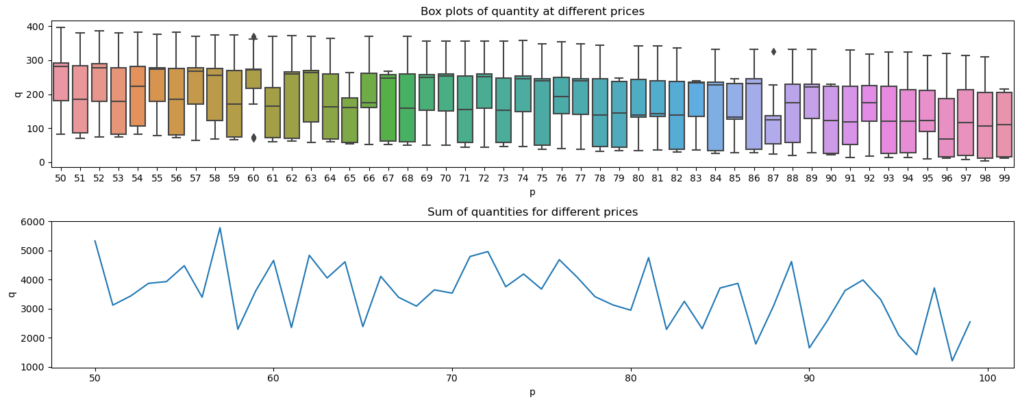
5.2. Visualize quantity over price trends

Below, we show the

• spread of quantity by price and

• also the sum of the quantity by price.

import matplotlib.pyplot as plt
import seaborn as sns

fig, ax = plt.subplots(2, 1, figsize=(15, 6))

sns.boxplot(df, x='p', y='q', ax=ax[0])
df.groupby(['p'])['q'].sum().plot(kind='line', ylabel='q', ax=ax[1])

ax[0].set_title('Box plots of quantity at different prices')
ax[1].set_title('Sum of quantities for different prices')

fig.tight_layout()

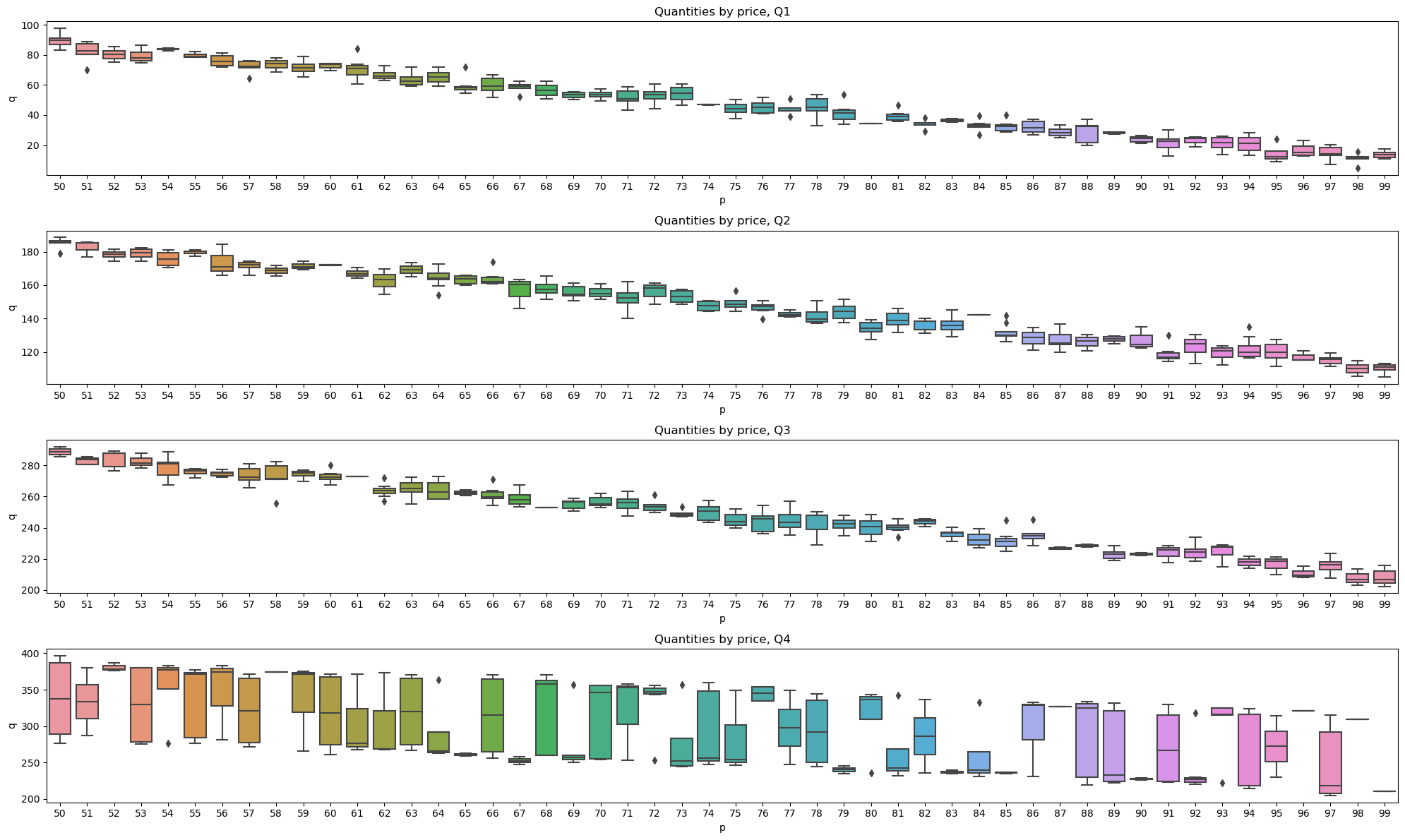
We can breakdown the data by quarters and observe the spread of quantities by price. In all quarters except the last, all quantities trend downward.

_temp = df.assign(quarter=lambda d: np.select([d.month < 4, d.month < 7, d.month < 10], [1, 2, 3], 4))

fig, axes = plt.subplots(4, 1, figsize=(20, 12))

for q, ax in zip([1, 2, 3, 4], np.ravel(axes)):
    sns.boxplot(
        _temp[_temp.quarter==q],
        x='p',
        y='q',
        ax=ax
    )

    ax.set_title(f'Quantities by price, Q{q}')

fig.tight_layout()

5.3. Demand data

The demand curve data will be grouped by price-month and quantities summed over.

demand_df = df.groupby(['p', 'month'])['q'].sum().to_frame().reset_index()
demand_df

	p	month	q
0	50	1	97.630858
1	50	2	170.132677
2	50	3	181.190757
3	50	4	367.611310
4	50	5	185.221784
...	...	...	...
461	99	6	443.360809
462	99	7	210.213176
463	99	8	818.645468
464	99	9	430.012356
465	99	10	210.007255

466 rows × 3 columns

5.4. Linear modeling

We can certainly model the demand curve using linear regression. As you can see below, the coefficient corresponding to price is -3.20. The mean absolute error MAE and weighted absolute percentage error WAPE are very big.

from sklearn.linear_model import LinearRegression

X = demand_df[['p', 'month']]
y = demand_df['q']

m = LinearRegression()
m.fit(X, y)

pd.Series([m.intercept_, m.coef_[0], m.coef_[1]], ['intercept', 'p', 'month'])

Intel(R) Extension for Scikit-learn* enabled (https://github.com/intel/scikit-learn-intelex)

intercept    221.907460
p             -3.199247
month         66.123215
dtype: float64

from sklearn.metrics import mean_absolute_error

mean_absolute_error(y, m.predict(X))

175.57064604298589

np.sum(np.abs(y - m.predict(X))) / np.sum(y)

0.4666900845671383

5.5. Non-linear modeling

In the non-linear modeling approach, we use a random forest to model the demand curve. Interestingly, month is more important than price. Also, using a non-linear model cuts the MAE and WAPE by over half of what we saw with the linear model. Let’s keep this model.

from sklearn.ensemble import RandomForestRegressor

X = demand_df[['p', 'month']]
y = demand_df['q']

m = RandomForestRegressor(n_jobs=-1, random_state=37, n_estimators=40)
m.fit(X, y)

pd.Series(m.feature_importances_, X.columns)

p        0.434937
month    0.565063
dtype: float64

mean_absolute_error(y, m.predict(X))

76.80770760690886

np.sum(np.abs(y - m.predict(X))) / np.sum(y)

0.20416508320929747

5.6. Visualizing quantities space

We can visualize the relationship between quantity (z-axis), price (x-axis) and month (y-axis). As you can tell, the surface is very complicated of how price and month interact to influence quantity.

x, y = np.meshgrid(np.arange(50, 100.1, 0.1), np.arange(1, 13, 1))
z = m.predict(pd.DataFrame([(_x, _y) for _x, _y in zip(np.ravel(x), np.ravel(y))], columns=['p', 'month'])).reshape(x.shape)

x.shape, y.shape, z.shape

((12, 501), (12, 501), (12, 501))

import plotly.graph_objects as go

fig = go.Figure(data=[go.Surface(
    x=x,
    y=y,
    z=z,
    colorscale='Viridis',
    opacity=0.5,
)])

fig.update_layout(
    title=r'$q = f(p, m_q)$',
    autosize=False,
    width=600,
    height=600,
    margin={'l': 65, 'r': 50, 'b': 65, 't': 90}
)
fig.update_xaxes(title='p')
fig.update_yaxes(title=r'$m_q$')

fig.show()

The contour plot is also complicated, but we can tell that the top region is where most of the high quantities reside from the interaction between month-quarter \(m_q\) and price \(p\).

fig = go.Figure(data =
    go.Contour(
        z=z,
        x=np.unique(x),
        y=np.unique(y),
        colorscale='Viridis'
    ))
fig.update_layout(
    title=r'$q = f(p, m_q)$',
    autosize=False,
    width=600,
    height=600,
    margin={'l': 65, 'r': 50, 'b': 65, 't': 90}
)
fig.update_xaxes(title='p')
fig.update_yaxes(title=r'$m_q$')

fig.show()

5.7. Maximize total revenue

Let’s try to maximize total revenue.

import optuna

optuna.logging.set_verbosity(optuna.logging.ERROR)

def rev_objective(trial, m):
    p = trial.suggest_float('p', 50, 100)
    month = trial.suggest_float('month', 1, 12)
    _df = pd.DataFrame([[p, month]], columns=['p', 'month'])
    z = m.predict(_df)
    q = z[0]

    r = p * q

    return r

study = optuna.create_study(**{
    'study_name': 'opt-revenue',
    'storage': 'sqlite:///_temp/opt-revenue.db',
    'load_if_exists': True,
    'direction': 'maximize',
    'sampler': optuna.samplers.TPESampler(seed=37),
    'pruner': optuna.pruners.MedianPruner(n_warmup_steps=10)
})

study.optimize(**{
    'func': lambda t: rev_objective(t, m),
    'n_trials': 1_000,
    'n_jobs': 6,
    'show_progress_bar': True
})

study.best_params

{'p': 88.4928117682058, 'month': 11.450811461657262}

study.best_value

103567.10107416332

_p = study.best_params['p']
_m = study.best_params['month']
_q = m.predict(pd.DataFrame([study.best_params]))[0]
_rev = _p * _q
_pft = (_p - 25) * _q

_rev_results = {
    'p': _p,
    'month': _m,
    'q': _q,
    'revenue': _rev,
    'profit': _pft
}

_rev_results

{'p': 88.4928117682058,
 'month': 11.450811461657262,
 'q': 1170.3447885173143,
 'revenue': 103567.10107416332,
 'profit': 74308.48136123046}

5.8. Maximize total profit

Let’s try to maximize profit.

def pft_objective(trial, m):
    p = trial.suggest_float('p', 50, 100)
    month = trial.suggest_float('month', 1, 12)
    _df = pd.DataFrame([[p, month]], columns=['p', 'month'])
    z = m.predict(_df)
    q = z[0]

    r = (p - 25) * q

    return r

study = optuna.create_study(**{
    'study_name': 'opt-profit',
    'storage': 'sqlite:///_temp/opt-profit.db',
    'load_if_exists': True,
    'direction': 'maximize',
    'sampler': optuna.samplers.TPESampler(seed=37),
    'pruner': optuna.pruners.MedianPruner(n_warmup_steps=10)
})

study.optimize(**{
    'func': lambda t: pft_objective(t, m),
    'n_trials': 1_000,
    'n_jobs': 6,
    'show_progress_bar': True
})

study.best_params

{'p': 93.48324856585506, 'month': 11.324420125907485}

study.best_value

75902.68836214142

_p = study.best_params['p']
_m = study.best_params['month']
_q = m.predict(pd.DataFrame([study.best_params]))[0]
_rev = _p * _q
_pft = (_p - 25) * _q

_pft_results = {
    'p': _p,
    'month': _m,
    'q': _q,
    'revenue': _rev,
    'profit': _pft
}

_pft_results

{'p': 93.48324856585506,
 'month': 11.324420125907485,
 'q': 1108.3394837666272,
 'revenue': 103611.17545630709,
 'profit': 75902.68836214142}

5.9. Maximize profit and revenue

Let’s try to maximize both profit and revenue.

def rev_pft_objective(trial, m):
    p = trial.suggest_float('p', 50, 100)
    month = trial.suggest_float('month', 1, 12)
    _df = pd.DataFrame([[p, month]], columns=['p', 'month'])
    z = m.predict(_df)
    q = z[0]

    pft = (p - 25) * q
    rev = p * q

    return rev, pft

study = optuna.create_study(**{
    'study_name': 'opt-rev-pft',
    'storage': 'sqlite:///_temp/opt-rev-pft.db',
    'load_if_exists': True,
    'directions': ['maximize', 'maximize'],
    'sampler': optuna.samplers.TPESampler(seed=37),
    'pruner': optuna.pruners.MedianPruner(n_warmup_steps=10)
})

study.optimize(**{
    'func': lambda t: rev_pft_objective(t, m),
    'n_trials': 1_000,
    'n_jobs': 6,
    'show_progress_bar': True
})

best = max(study.best_trials, key=lambda t: (t.values[0], t.values[1]))

best

FrozenTrial(number=421, state=TrialState.COMPLETE, values=[103523.72177069388, 75815.2346765282], datetime_start=datetime.datetime(2023, 9, 7, 1, 15, 4, 325108), datetime_complete=datetime.datetime(2023, 9, 7, 1, 15, 5, 8747), params={'p': 93.40434342271607, 'month': 10.965941774282502}, user_attrs={}, system_attrs={}, intermediate_values={}, distributions={'p': FloatDistribution(high=100.0, log=False, low=50.0, step=None), 'month': FloatDistribution(high=12.0, log=False, low=1.0, step=None)}, trial_id=422, value=None)

best.params

{'p': 93.40434342271607, 'month': 10.965941774282502}

best.values

[103523.72177069388, 75815.2346765282]

m.predict(pd.DataFrame([best.params]))[0]

1108.3394837666272

_p = best.params['p']
_m = best.params['month']
_q = m.predict(pd.DataFrame([best.params]))[0]
_rev = _p * _q
_pft = (_p - 25) * _q

_revpft_results = {
    'p': _p,
    'month': _m,
    'q': _q,
    'revenue': _rev,
    'profit': _pft
}

_revpft_results

{'p': 93.40434342271607,
 'month': 10.965941774282502,
 'q': 1108.3394837666272,
 'revenue': 103523.72177069388,
 'profit': 75815.2346765282}

5.10. Maximize quantity, revenue and profit

def q_rev_pft_objective(trial, m):
    p = trial.suggest_float('p', 50, 100)
    month = trial.suggest_float('month', 1, 12)
    _df = pd.DataFrame([[p, month]], columns=['p', 'month'])
    z = m.predict(_df)
    q = z[0]

    pft = (p - 25) * q
    rev = p * q

    return q, rev, pft

study = optuna.create_study(**{
    'study_name': 'opt-q-rev-pft',
    'storage': 'sqlite:///_temp/opt-q-rev-pft.db',
    'load_if_exists': True,
    'directions': ['maximize', 'maximize', 'maximize'],
    'sampler': optuna.samplers.TPESampler(seed=37),
    'pruner': optuna.pruners.MedianPruner(n_warmup_steps=10)
})

study.optimize(**{
    'func': lambda t: q_rev_pft_objective(t, m),
    'n_trials': 1_000,
    'n_jobs': 6,
    'show_progress_bar': True
})

best = max(study.best_trials, key=lambda t: (t.values[0], t.values[1]))

best.params

{'p': 50.184457378381126, 'month': 11.04879031751835}

best.values

[1640.2904172779429, 82317.08453405192, 41309.82410210335]

m.predict(pd.DataFrame([best.params]))[0]

1640.2904172779429

_p = best.params['p']
_m = best.params['month']
_q = m.predict(pd.DataFrame([best.params]))[0]
_rev = _p * _q
_pft = (_p - 25) * _q

_qrp_results = {
    'p': _p,
    'month': _m,
    'q': _q,
    'revenue': _rev,
    'profit': _pft
}

_qrp_results

{'p': 50.184457378381126,
 'month': 11.04879031751835,
 'q': 1640.2904172779429,
 'revenue': 82317.08453405192,
 'profit': 41309.82410210335}

The best parameters when maximizing for revenue, profit, revenue and profit and quantity, revenue and profit are shown below.

pd.DataFrame([
    _rev_results,
    _pft_results,
    _revpft_results,
    _qrp_results,
], index=['max_revenue', 'max_profit', 'max_both', 'max_all'])

	p	month	q	revenue	profit
max_revenue	88.492812	11.450811	1170.344789	103567.101074	74308.481361
max_profit	93.483249	11.324420	1108.339484	103611.175456	75902.688362
max_both	93.404343	10.965942	1108.339484	103523.721771	75815.234677
max_all	50.184457	11.048790	1640.290417	82317.084534	41309.824102

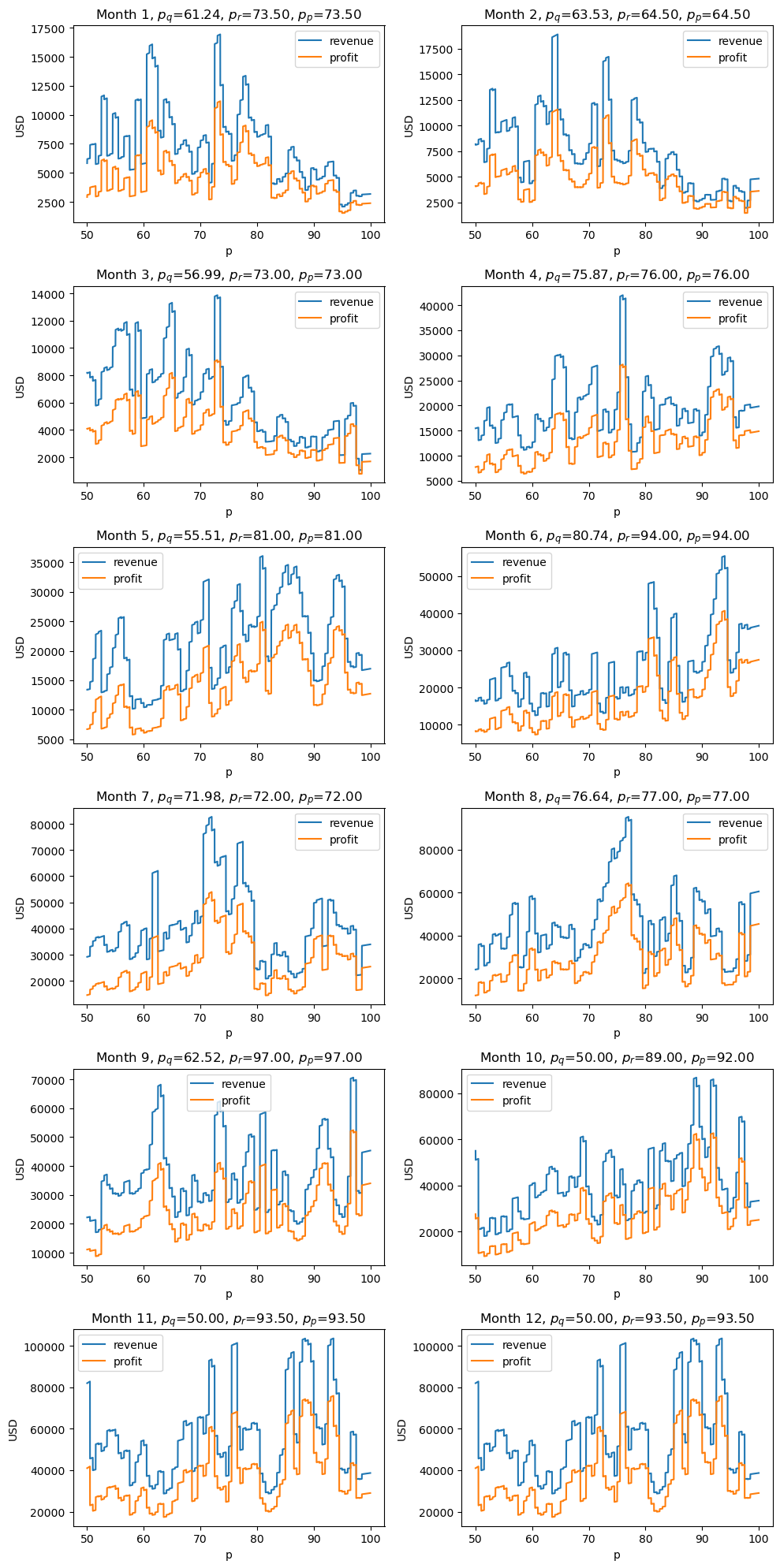
5.11. Visualize monthly revenue and profit

Below, we visualize expected revenue and profit over price for each month.

• \(p_q\) is the price that optimizes the quantity

• \(p_r\) is the price that optimizes the revenue

• \(p_p\) is the price that optimizes the profit

def get_estimate(month):
    return pd.DataFrame({'p': np.arange(50, 100.01, 0.01), 'month': month}) \
        .assign(
            q=lambda d: m.predict(d),
            revenue=lambda d: d['p'] * d['q'],
            profit=lambda d: (d['p'] - 25) * d['q']
        ) \
        .set_index(['p']) \
        [['q', 'revenue', 'profit']]

fig, axes = plt.subplots(6, 2, figsize=(10, 20))

for month, ax in zip(np.arange(1, 13, 1), np.ravel(axes)):
    _df = get_estimate(month)
    _df[['revenue', 'profit']].plot(kind='line', ax=ax)

    _p_qty = _df.sort_values(['q'], ascending=False).index[0]
    _p_rev = _df.sort_values(['revenue'], ascending=False).index[0]
    _p_pft = _df.sort_values(['profit'], ascending=False).index[0]

    ax.set_title(rf'Month {month}, $p_q$={_p_qty:.2f}, $p_r$={_p_rev:.2f}, $p_p$={_p_pft:.2f}')
    ax.set_ylabel('USD')

fig.tight_layout()

5.12. Visualizing revenue

Because we love interactive surface plots, let’s plot expected total revenue (z-axis) against price (x-axis) and month (y-axis).

x, y = np.meshgrid(np.arange(50, 100.1, 0.1), np.arange(1, 13, 1))
z = m.predict(pd.DataFrame([(_x, _y) for _x, _y in zip(np.ravel(x), np.ravel(y))], columns=['p', 'month'])).reshape(x.shape)
r = x * z
t = (x - 25) * z

((12, 501), (12, 501), (12, 501), (12, 501), (12, 501))

fig = go.Figure(data=[go.Surface(
    x=x,
    y=y,
    z=r,
    colorscale='Viridis',
    opacity=0.5,
)])

fig.update_layout(
    title=r'$r = qp = f(p, m_q) p$',
    autosize=False,
    width=600,
    height=600,
    margin={'l': 65, 'r': 50, 'b': 65, 't': 90}
)
fig.update_xaxes(title='p')
fig.update_yaxes(title=r'$m_q$')

fig.show()

5.13. Visualizing profit

This next surface plot is of expected total profit (z-axis) against price (x-axis) and month (y-axis).

fig = go.Figure(data=[go.Surface(
    x=x,
    y=y,
    z=t,
    colorscale='Viridis',
    opacity=0.5,
)])

fig.update_layout(
    title=r'$t = q(p - c) = f(p, m_q) (p - c)$',
    autosize=False,
    width=600,
    height=600,
    margin={'l': 65, 'r': 50, 'b': 65, 't': 90}
)
fig.update_xaxes(title='p')
fig.update_yaxes(title=r'$m_q$')

fig.show()