2. Massey’s Method

Massey’s Method refers to Kenneth Massey’s method for ranking sport teams. Denote the following.

• \(n\) is the number of teams

• \(m\) is the number games played (only 2 teams can play in a game)

• \(X\) is a \(n\) x \(m\) matrix where columns corresponding to teams and rows correspond to games

  • Each row of \(X\) is sparse (mostly zeros)

  • For each row, 1 is placed in the column corresponding to the winning team

  • For each row, -1 is placed in the column corresponding to the losing team

• \(r\) is a \(n\) x 1 vector corresponding to the rating of each team

  • \(r\) is what will be estimated

• \(y\) is a \(n\) x 1 vector corresponding to the margins of victory

Then, we are trying to solve

\(Xr = y\)

Futhermore, denote coefficient matrix \(M\) as \(M = X^TX\). Thus, \(M\) will be \(n\) x \(n\) and

• the diagonal elements \(M_{ii}\) of \(M\) will be the number of games played by the i-th team,

• the off-diagonal elements \(M_{ij}\) will be the negation of the number of times the i-th team played the j-th team.

Instead of solving \(Xr = y\), then we can solve the following,

\(Mr = p\),

where \(p = X^Ty\).

2.1. Data

Let’s illustrate Massey’s Method using data from the NCAAF ACC conference for the year 2005. Below, t1 and t2 are the 2 teams playing and s1 and s2 are the scores corresponding to t1 and t2. There is no information on who was at home or away.

import pandas as pd

f_df = pd.read_csv('./ranking/acc-2005-ncaaf.csv')
f_df

	t1	t2	s1	s2
0	Duke	Miami	7	52
1	Duke	UNC	21	24
2	Duke	UVA	7	38
3	Duke	VT	0	45
4	Miami	UNC	34	16
5	Miami	UVA	25	17
6	Miami	VT	27	7
7	UNC	UVA	7	5
8	UNC	VT	3	30
9	UVA	VT	14	52

We can swap the teams and scores and get a view like the following.

r_df = pd.DataFrame([{'t1': r.t2, 't2': r.t1, 's1': r.s2, 's2': r.s1} for _, r in f_df.iterrows()])

game_df = pd.concat([f_df, r_df]).reset_index(drop=True)
game_df['differential'] = game_df.s1 - game_df.s2
game_df.sort_values(['t1', 't2'])

	t1	t2	s1	s2	differential
0	Duke	Miami	7	52	-45
1	Duke	UNC	21	24	-3
2	Duke	UVA	7	38	-31
3	Duke	VT	0	45	-45
10	Miami	Duke	52	7	45
4	Miami	UNC	34	16	18
5	Miami	UVA	25	17	8
6	Miami	VT	27	7	20
11	UNC	Duke	24	21	3
14	UNC	Miami	16	34	-18
7	UNC	UVA	7	5	2
8	UNC	VT	3	30	-27
12	UVA	Duke	38	7	31
15	UVA	Miami	17	25	-8
17	UVA	UNC	5	7	-2
9	UVA	VT	14	52	-38
13	VT	Duke	45	0	45
16	VT	Miami	7	27	-20
18	VT	UNC	30	3	27
19	VT	UVA	52	14	38

import matplotlib.pyplot as plt
import seaborn as sns

plt.style.use('ggplot')

fig, ax = plt.subplots(figsize=(10, 4))

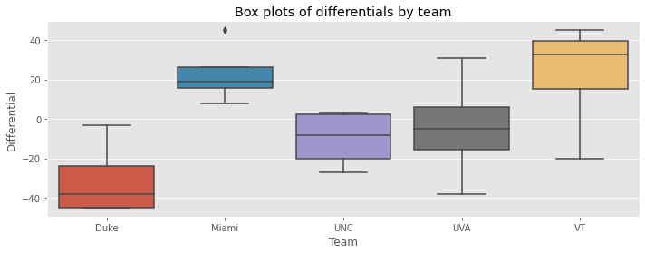
_ = sns.boxplot(x='t1', y='differential', data=game_df, ax=ax)
_ = ax.set_title('Box plots of differentials by team')
_ = ax.set_xlabel('Team')
_ = ax.set_ylabel('Differential')

plt.tight_layout()

2.2. Ranking from ratings

A \(n\) x \(n\) matrix of point differential for each team can be created as follows. In the matrix below, UNC

• won Duke by 3 points,

• lost to Miami by 18 points,

• win UVA by 2 points, and

• lost to VT by 27 points.

When a team wins, the number in this matrix is positive, and when a team loses, the number in this matrix is negative.

import numpy as np

def get_differential(t1, t2):
    if t1 == t2:
        return np.nan
    s = game_df[(game_df.t1 == t1) & (game_df.t2 == t2)].iloc[0]
    return s.s1 - s.s2

teams = sorted(list(set(game_df.t1) | set(game_df.t2)))
differentials = [[get_differential(t1, t2) for t2 in teams] for t1 in teams]

diff_df = pd.DataFrame(differentials, index=teams, columns=teams)
diff_df

	Duke	Miami	UNC	UVA	VT
Duke	NaN	-45.0	-3.0	-31.0	-45.0
Miami	45.0	NaN	18.0	8.0	20.0
UNC	3.0	-18.0	NaN	2.0	-27.0
UVA	31.0	-8.0	-2.0	NaN	-38.0
VT	45.0	-20.0	27.0	38.0	NaN

From this point differential matrix, we can then compute the total point differential (sum across the columns) and the number of wins (positive scores) and losses (negative scores).

stat_df = pd.DataFrame({
    'differential': diff_df.sum(axis=1),
    'wins': diff_df.apply(lambda r: len(r[r > 0]), axis=1),
    'losses': diff_df.apply(lambda r: len(r[r < 0]), axis=1)
})

stat_df

	differential	wins	losses
Duke	-124.0	0	4
Miami	91.0	4	0
UNC	-40.0	2	2
UVA	-17.0	1	3
VT	90.0	3	1

If we let the sum of the point differentials be the ratings, then the ranking produced is as follows where Miami is first and Duke is last.

stat_df.differential.sort_values(ascending=False)

Miami     91.0
VT        90.0
UVA      -17.0
UNC      -40.0
Duke    -124.0
Name: differential, dtype: float64

We can also let the number of wins be the ratings, and Miami is still first and Duke is last.

stat_df.wins.sort_values(ascending=False)

Miami    4
VT       3
UNC      2
UVA      1
Duke     0
Name: wins, dtype: int64

Let’s compare the ranking by point differential and wins. Notice that the rankings are nearly identical, except that UVA and UNC switch places?

pd.DataFrame({
    'by_differential': stat_df.differential.sort_values(ascending=False).index,
    'by_wins': stat_df.wins.sort_values(ascending=False).index
})

	by_differential	by_wins
0	Miami	Miami
1	VT	VT
2	UVA	UNC
3	UNC	UVA
4	Duke	Duke

2.3. Xr = y

Let’s build or \(X\) matrix.

def get_vector(r):
    v = [0 for i in range(len(teams))]

    if r.s1 > r.s2:
        v[t2i[r.t1]] = 1
        v[t2i[r.t2]] = -1
    else:
        v[t2i[r.t1]] = -1
        v[t2i[r.t2]] = 1
    return v

t2i = {t: i for i, t in enumerate(teams)}

X = pd.DataFrame([get_vector(r) for _, r in f_df.iterrows()], columns=teams)
X

	Duke	Miami	UNC	UVA	VT
0	-1	1	0	0	0
1	-1	0	1	0	0
2	-1	0	0	1	0
3	-1	0	0	0	1
4	0	1	-1	0	0
5	0	1	0	-1	0
6	0	1	0	0	-1
7	0	0	1	-1	0
8	0	0	-1	0	1
9	0	0	0	-1	1

Notice that \(X^TX = M\).

X.T.dot(X)

	Duke	Miami	UNC	UVA	VT
Duke	4	-1	-1	-1	-1
Miami	-1	4	-1	-1	-1
UNC	-1	-1	4	-1	-1
UVA	-1	-1	-1	4	-1
VT	-1	-1	-1	-1	4

Our \(y\) will be the point differential.

y = f_df.s1 - f_df.s2
y

0   -45
1    -3
2   -31
3   -45
4    18
5     8
6    20
7     2
8   -27
9   -38
dtype: int64

We will not attempt to learn the ratings using linear regression.

from sklearn.linear_model import LinearRegression

model = LinearRegression()
model.fit(X, y)
model.intercept_, model.coef_

(4.100000000000035, array([ 28.08,  -3.08,   1.6 ,   1.04, -27.64]))

The ratings are the coefficients (see below where we negate them). However, because \(m >> n\), the linear system is highly overdetermined and inconsistent.

sorted(list(zip(teams, -model.coef_)), key=lambda tup: tup[1], reverse=True)

[('VT', 27.640000000000022),
 ('Miami', 3.080000000000026),
 ('UVA', -1.0400000000000234),
 ('UNC', -1.5999999999999974),
 ('Duke', -28.08000000000003)]

Note how Miami is undefeated, but still in second place? It is likely VT came in first place since their point differentials average higher. In most sports ranking system, point differentials are take out of consideration because teams with a high lead may stop scoring points as a matter of sportsmanship.

2.4. Mr = p

Here, we will estimating the ratings and thus the ranking using the coefficient matrix \(M\).

def get_games_played(t1, t2):
    if t1 == t2:
        return f_df[(f_df.t1 == t1) | (f_df.t2 == t2)].shape[0]
    else:
        q1 = (f_df.t1 == t1) & (f_df.t2 == t2)
        q2 = (f_df.t1 == t2) & (f_df.t2 == t1)
        q = q1 | q2
        return -f_df[q].shape[0]

mat = [[get_games_played(t1, t2) for t2 in teams] for t1 in teams]
mat

[[4, -1, -1, -1, -1],
 [-1, 4, -1, -1, -1],
 [-1, -1, 4, -1, -1],
 [-1, -1, -1, 4, -1],
 [-1, -1, -1, -1, 4]]

To ensure that \(M\) has full rank, we will convert the last row to all 1’s.

mat[-1] = [1 for _ in range(len(mat[-1]))]
mat

[[4, -1, -1, -1, -1],
 [-1, 4, -1, -1, -1],
 [-1, -1, 4, -1, -1],
 [-1, -1, -1, 4, -1],
 [1, 1, 1, 1, 1]]

Our final \(M\) looks like the following.

M = pd.DataFrame(mat, index=teams, columns=teams)
M

	Duke	Miami	UNC	UVA	VT
Duke	4	-1	-1	-1	-1
Miami	-1	4	-1	-1	-1
UNC	-1	-1	4	-1	-1
UVA	-1	-1	-1	4	-1
VT	1	1	1	1	1

Our \(p\) looks like the following.

p = stat_df.differential
p

Duke    -124.0
Miami     91.0
UNC      -40.0
UVA      -17.0
VT        90.0
Name: differential, dtype: float64

Applying linear regression and sorting the ratings (coefficients), we get the final ranking below.

model = LinearRegression()
model.fit(M, p)
model.intercept_, model.coef_

(8.881784197001252e-15, array([-6.8, 36.2, 10. , 14.6, 36. ]))

sorted(list(zip(teams, model.coef_)), key=lambda tup: tup[1], reverse=True)

[('Miami', 36.2),
 ('VT', 36.00000000000002),
 ('UVA', 14.599999999999998),
 ('UNC', 9.999999999999998),
 ('Duke', -6.799999999999999)]

2.5. NBA 2021

Let’s apply Massey’s Method to the NBA for the 2021 season and games up to Thanksgiving.

def get_nba():
    x = pd.read_csv('./nba/2021.csv')\
        .rename(columns={
            'a_team': 't1',
            'h_team': 't2',
            'a_score': 's1',
            'h_score': 's2'})
    x = x[x.preseason == False]\
        .drop(columns=['preseason'])\
        .reset_index(drop=True)
    return x

def get_nfl():
    x = pd.read_csv('./nfl/2021.csv')\
        .rename(columns={
            'team1': 't1',
            'team2': 't2',
            'score1': 's1',
            'score2': 's2'})\
        .drop(columns=['week'])
    x['t1'] = x['t1'].apply(lambda s: s.strip())
    x['t2'] = x['t2'].apply(lambda s: s.strip())

    return x

def get_X(df):
    def get_vector(r):
        v = [0 for i in range(len(teams))]

        if r.s1 > r.s2:
            v[t2i[r.t1]] = 1
            v[t2i[r.t2]] = -1
        else:
            v[t2i[r.t1]] = -1
            v[t2i[r.t2]] = 1
        return v

    teams = sorted(list(set(df.t1) | set(df.t2)))
    t2i = {t: i for i, t in enumerate(teams)}

    X = pd.DataFrame([get_vector(r) for _, r in df.iterrows()], columns=teams)
    X = X.T.dot(X)
    X.iloc[-1,:] = 1

    return X

def get_y(df):
    def get_diff(t):
        a = df[df.t1 == t]
        b = df[df.t2 == t]

        c = a.s1 - a.s2
        d = b.s2 - b.s1

        return c.sum() + d.sum()

    teams = sorted(list(set(df.t1) | set(df.t2)))
    diffs = [get_diff(t) for t in teams]

    return pd.Series(diffs, index=teams)

def get_Xy(df):
    return get_X(df), get_y(df)

X, y = get_Xy(get_nba())

model = LinearRegression()
model.fit(X, y)

pd.DataFrame(zip(X.index, model.coef_), columns=['Team', 'Rating'])\
    .sort_values('Rating', ascending=False)

	Team	Rating
28	Warriors	12.899850
10	Jazz	8.549796
24	Suns	6.744632
8	Heat	6.488263
16	Nets	4.254646
2	Bulls	4.235154
5	Clippers	3.792290
7	Hawks	3.338752
18	Pacers	3.138730
27	Trail Blazers	2.456361
0	76ers	2.100543
1	Bucks	1.999356
3	Cavaliers	1.429301
26	Timberwolves	1.276979
9	Hornets	1.227789
29	Wizards	1.180180
21	Raptors	1.055674
17	Nuggets	0.755934
4	Celtics	0.579776
11	Kings	0.089514
12	Knicks	-0.306992
15	Mavericks	-0.688728
13	Lakers	-3.357641
23	Spurs	-3.433295
6	Grizzlies	-4.525625
19	Pelicans	-4.916126
25	Thunder	-5.150785
20	Pistons	-7.552551
22	Rockets	-8.788710
14	Magic	-9.818479

2.6. NFL

Let’s apply Massey’s Method to the NFL for the 2021 season and games up to Thanksgiving.

X, y = get_Xy(get_nfl())

model = LinearRegression()
model.fit(X, y)

pd.DataFrame(zip(X.index, model.coef_), columns=['Team', 'Rating'])\
    .sort_values('Rating', ascending=False)

	Team	Rating
3	Bills	8.425259
7	Cardinals	8.235687
21	Patriots	6.349719
6	Buccaneers	6.321022
11	Cowboys	5.819441
10	Colts	3.115332
9	Chiefs	2.706593
29	Titans	2.584503
23	Rams	2.472228
13	Eagles	1.696797
0	49ers	1.565063
19	Packers	1.443518
25	Saints	0.808172
30	Vikings	0.737758
8	Chargers	-0.551756
2	Bengals	-0.607977
26	Seahawks	-0.880815
24	Ravens	-1.608072
20	Panthers	-1.742287
4	Broncos	-2.431469
5	Browns	-2.723871
31	Washington	-3.649900
27	Steelers	-3.707054
22	Raiders	-5.414601
15	Giants	-6.524430
12	Dolphins	-8.305769
1	Bears	-9.322540
16	Jaguars	-10.338981
28	Texans	-11.365255
18	Lions	-12.281915
14	Falcons	-12.409125
17	Jets	-14.139647