4. Chernoff Faces, Inception v3
Here we use the Inception v3 convolutional neural network (CNN) to classify Chernoff faces. We will judge its performance with the receiver operating characteristic (ROC) and precision-recall (PR) curves.
4.1. Training and validation
Below is boilerplate code to learn from data.
[1]:
import torch
import torch.nn as nn
import torch.optim as optim
from torch.optim import lr_scheduler
import numpy as np
import torchvision
from torchvision import datasets, models, transforms
import matplotlib.pyplot as plt
import time
import os
import copy
from collections import namedtuple
from sklearn.metrics import multilabel_confusion_matrix
from collections import namedtuple
import random

def get_dataloaders(input_size=256, batch_size=4):
    data_transforms = {
        'train': transforms.Compose([
            transforms.Resize(input_size),
            transforms.CenterCrop(input_size),
            transforms.ToTensor(),
            transforms.Normalize(mean=[0.485, 0.456, 0.406], std=[0.229, 0.224, 0.225])
        ]),
        'test': transforms.Compose([
            transforms.Resize(input_size),
            transforms.CenterCrop(input_size),
            transforms.ToTensor(),
            transforms.Normalize(mean=[0.485, 0.456, 0.406], std=[0.229, 0.224, 0.225])
        ]),
        'valid': transforms.Compose([
            transforms.Resize(input_size),
            transforms.CenterCrop(input_size),
            transforms.ToTensor(),
            transforms.Normalize(mean=[0.485, 0.456, 0.406], std=[0.229, 0.224, 0.225])
        ])
    }

    shuffles = {
        'train': True,
        'test': True,
        'valid': False
    }

    data_dir = './faces'
    samples = ['train', 'test', 'valid']
    image_datasets = { x: datasets.ImageFolder(os.path.join(data_dir, x), transform=data_transforms[x]) for x in samples }
    dataloaders = { x: torch.utils.data.DataLoader(image_datasets[x], batch_size=batch_size, shuffle=shuffles[x], num_workers=4)
                   for x in samples }
    dataset_sizes = { x: len(image_datasets[x]) for x in samples }
    class_names = image_datasets['train'].classes

    return dataloaders, dataset_sizes, class_names, len(class_names)

def train_model(model, criterion, optimizer, scheduler, dataloaders, dataset_sizes, num_epochs=25, is_inception=False):
    since = time.time()

    best_model_wts = copy.deepcopy(model.state_dict())
    best_acc = 0.0

    for epoch in range(num_epochs):
        results = []
        # Each epoch has a training and validation phase
        for phase in ['train', 'test']:
            if phase == 'train':
                optimizer.step()
                scheduler.step()
                model.train()  # Set model to training mode
            else:
                model.eval()   # Set model to evaluate mode

            running_loss = 0.0
            running_corrects = 0

            # Iterate over data.
            for inputs, labels in dataloaders[phase]:
                inputs = inputs.to(device)
                labels = labels.to(device)

                # zero the parameter gradients
                optimizer.zero_grad()

                # forward
                # track history if only in train
                with torch.set_grad_enabled(phase == 'train'):
                    if is_inception and phase == 'train':
                        outputs, aux_outputs = model(inputs)
                        loss1 = criterion(outputs, labels)
                        loss2 = criterion(aux_outputs, labels)
                        loss = loss1 + 0.4*loss2
                    else:
                        outputs = model(inputs)
                        loss = criterion(outputs, labels)

                    _, preds = torch.max(outputs, 1)

                    # backward + optimize only if in training phase
                    if phase == 'train':
                        loss.backward()
                        optimizer.step()

                # statistics
                running_loss += loss.item() * inputs.size(0)
                running_corrects += torch.sum(preds == labels.data)

            epoch_loss = running_loss / dataset_sizes[phase]
            epoch_acc = running_corrects.double() / dataset_sizes[phase]

            result = Result(phase, epoch_loss, float(str(epoch_acc.cpu().numpy())))
            results.append(result)

            # deep copy the model
            if phase == 'test' and epoch_acc > best_acc:
                best_acc = epoch_acc
                best_model_wts = copy.deepcopy(model.state_dict())

        results = ['{} loss: {:.4f} acc: {:.4f}'.format(r.phase, r.loss, r.acc) for r in results]
        results = ' | '.join(results)
        print('Epoch {}/{} | {}'.format(epoch, num_epochs - 1, results))

    time_elapsed = time.time() - since
    print('Training complete in {:.0f}m {:.0f}s'.format(
        time_elapsed // 60, time_elapsed % 60))
    print('Best val Acc: {:4f}'.format(best_acc))

    # load best model weights
    model.load_state_dict(best_model_wts)
    return model

def get_metrics(model, dataloaders, class_names):
    y_true = []
    y_pred = []
    was_training = model.training
    model.eval()

    with torch.no_grad():
        for i, (inputs, labels) in enumerate(dataloaders['valid']):
            inputs = inputs.to(device)
            labels = labels.to(device)
            cpu_labels = labels.cpu().numpy()

            outputs = model(inputs)
            _, preds = torch.max(outputs, 1)

            for j in range(inputs.size()[0]):
                cpu_label = f'{cpu_labels[j]:02}'
                clazz_name = class_names[preds[j]]

                y_true.append(cpu_label)
                y_pred.append(clazz_name)


        model.train(mode=was_training)

    cmatrices = multilabel_confusion_matrix(y_true, y_pred, labels=class_names)
    metrics = []
    for clazz in range(len(cmatrices)):
        cmatrix = cmatrices[clazz]
        tn, fp, fn, tp = cmatrix[0][0], cmatrix[0][1], cmatrix[1][0], cmatrix[1][1]
        sen = tp / (tp + fn)
        spe = tn / (tn + fp)
        acc = (tp + tn) / (tp + fp + fn + tn)
        f1 = (2.0 * tp) / (2 * tp + fp + fn)
        mcc = (tp * tn - fp * fn) / np.sqrt((tp + fp) * (tp + fn) * (tn + fp) * (tn + fn))
        metric = Metric(clazz, tn, fp, fn, tp, sen, spe, acc, f1, mcc)
        metrics.append(metric)

    return metrics

def print_metrics(metrics):
    for m in metrics:
        print('{}: sen = {:.5f}, spe = {:.5f}, acc = {:.5f}, f1 = {:.5f}, mcc = {:.5f}'
              .format(m.clazz, m.sen, m.spe, m.acc, m.f1, m.mcc))

random.seed(1299827)
torch.manual_seed(1299827)
torch.backends.cudnn.deterministic = True
torch.backends.cudnn.benchmark = False

device = torch.device("cuda:0" if torch.cuda.is_available() else "cpu")
print('device = {}'.format(device))

Result = namedtuple('Result', 'phase loss acc')
Metric = namedtuple('Metric', 'clazz tn fp fn tp sen spe acc f1 mcc')
device = cuda:0
4.1.1. Train
[2]:
dataloaders, dataset_sizes, class_names, num_classes = get_dataloaders(input_size=299)
model = models.inception_v3(pretrained=True)
model.AuxLogits.fc = nn.Linear(model.AuxLogits.fc.in_features, num_classes)
model.fc = nn.Linear(model.fc.in_features, num_classes)
is_inception = True

model = model.to(device)
criterion = nn.CrossEntropyLoss()
optimizer = optim.SGD(model.parameters(), lr=0.001, momentum=0.9)
scheduler = lr_scheduler.StepLR(optimizer, step_size=7, gamma=0.1)

model = train_model(model, criterion, optimizer, scheduler, dataloaders, dataset_sizes, num_epochs=50, is_inception=is_inception)

print_metrics(get_metrics(model, dataloaders, class_names))
Epoch 0/49 | train loss: 0.7796 acc: 0.7778 | test loss: 0.7683 acc: 0.7600
Epoch 1/49 | train loss: 0.4087 acc: 0.8778 | test loss: 0.5574 acc: 0.8800
Epoch 2/49 | train loss: 0.3773 acc: 0.9111 | test loss: 0.4648 acc: 0.8300
Epoch 3/49 | train loss: 0.2763 acc: 0.9378 | test loss: 0.1745 acc: 0.9100
Epoch 4/49 | train loss: 0.2399 acc: 0.9667 | test loss: 0.3975 acc: 0.8800
Epoch 5/49 | train loss: 0.1584 acc: 0.9844 | test loss: 0.3012 acc: 0.9100
Epoch 6/49 | train loss: 0.1382 acc: 0.9822 | test loss: 0.3088 acc: 0.9100
Epoch 7/49 | train loss: 0.0690 acc: 0.9956 | test loss: 0.2584 acc: 0.9200
Epoch 8/49 | train loss: 0.0806 acc: 0.9889 | test loss: 0.2482 acc: 0.9200
Epoch 9/49 | train loss: 0.0898 acc: 0.9956 | test loss: 0.2575 acc: 0.9300
Epoch 10/49 | train loss: 0.0577 acc: 1.0000 | test loss: 0.2542 acc: 0.9200
Epoch 11/49 | train loss: 0.0769 acc: 0.9933 | test loss: 0.3179 acc: 0.9100
Epoch 12/49 | train loss: 0.0677 acc: 0.9933 | test loss: 0.2830 acc: 0.9200
Epoch 13/49 | train loss: 0.0656 acc: 0.9956 | test loss: 0.2517 acc: 0.9300
Epoch 14/49 | train loss: 0.0694 acc: 0.9956 | test loss: 0.2529 acc: 0.9200
Epoch 15/49 | train loss: 0.0730 acc: 0.9956 | test loss: 0.2968 acc: 0.9200
Epoch 16/49 | train loss: 0.0470 acc: 1.0000 | test loss: 0.2380 acc: 0.9300
Epoch 17/49 | train loss: 0.0534 acc: 0.9956 | test loss: 0.3000 acc: 0.9100
Epoch 18/49 | train loss: 0.0564 acc: 0.9956 | test loss: 0.2472 acc: 0.9300
Epoch 19/49 | train loss: 0.0326 acc: 1.0000 | test loss: 0.2404 acc: 0.9400
Epoch 20/49 | train loss: 0.0325 acc: 1.0000 | test loss: 0.2609 acc: 0.9200
Epoch 21/49 | train loss: 0.0496 acc: 0.9956 | test loss: 0.2419 acc: 0.9200
Epoch 22/49 | train loss: 0.0455 acc: 1.0000 | test loss: 0.2516 acc: 0.9200
Epoch 23/49 | train loss: 0.0620 acc: 0.9933 | test loss: 0.2415 acc: 0.9200
Epoch 24/49 | train loss: 0.0544 acc: 0.9911 | test loss: 0.2544 acc: 0.9200
Epoch 25/49 | train loss: 0.0614 acc: 0.9978 | test loss: 0.2409 acc: 0.9200
Epoch 26/49 | train loss: 0.0431 acc: 1.0000 | test loss: 0.2501 acc: 0.9400
Epoch 27/49 | train loss: 0.0461 acc: 1.0000 | test loss: 0.2444 acc: 0.9200
Epoch 28/49 | train loss: 0.0660 acc: 0.9956 | test loss: 0.2394 acc: 0.9200
Epoch 29/49 | train loss: 0.0652 acc: 0.9956 | test loss: 0.2580 acc: 0.9200
Epoch 30/49 | train loss: 0.0519 acc: 0.9956 | test loss: 0.2343 acc: 0.9200
Epoch 31/49 | train loss: 0.0488 acc: 0.9956 | test loss: 0.2350 acc: 0.9300
Epoch 32/49 | train loss: 0.0442 acc: 0.9956 | test loss: 0.2327 acc: 0.9300
Epoch 33/49 | train loss: 0.0610 acc: 0.9978 | test loss: 0.2714 acc: 0.9200
Epoch 34/49 | train loss: 0.0549 acc: 0.9933 | test loss: 0.2817 acc: 0.9000
Epoch 35/49 | train loss: 0.0882 acc: 0.9933 | test loss: 0.2376 acc: 0.9400
Epoch 36/49 | train loss: 0.0526 acc: 0.9978 | test loss: 0.2401 acc: 0.9200
Epoch 37/49 | train loss: 0.0647 acc: 0.9956 | test loss: 0.2611 acc: 0.9200
Epoch 38/49 | train loss: 0.0355 acc: 1.0000 | test loss: 0.2455 acc: 0.9200
Epoch 39/49 | train loss: 0.0578 acc: 0.9956 | test loss: 0.2681 acc: 0.9200
Epoch 40/49 | train loss: 0.0608 acc: 0.9956 | test loss: 0.2788 acc: 0.9200
Epoch 41/49 | train loss: 0.0516 acc: 0.9978 | test loss: 0.2521 acc: 0.9200
Epoch 42/49 | train loss: 0.0456 acc: 0.9978 | test loss: 0.2362 acc: 0.9200
Epoch 43/49 | train loss: 0.0684 acc: 0.9911 | test loss: 0.2298 acc: 0.9200
Epoch 44/49 | train loss: 0.0522 acc: 1.0000 | test loss: 0.2652 acc: 0.9300
Epoch 45/49 | train loss: 0.0654 acc: 0.9933 | test loss: 0.2701 acc: 0.9300
Epoch 46/49 | train loss: 0.0745 acc: 0.9978 | test loss: 0.2619 acc: 0.9200
Epoch 47/49 | train loss: 0.0715 acc: 0.9978 | test loss: 0.2437 acc: 0.9200
Epoch 48/49 | train loss: 0.0540 acc: 0.9978 | test loss: 0.2467 acc: 0.9200
Epoch 49/49 | train loss: 0.0687 acc: 0.9911 | test loss: 0.2810 acc: 0.9200
Training complete in 5m 49s
Best val Acc: 0.940000
0: sen = 1.00000, spe = 1.00000, acc = 1.00000, f1 = 1.00000, mcc = 1.00000
1: sen = 1.00000, spe = 0.97333, acc = 0.98000, f1 = 0.96154, mcc = 0.94933
2: sen = 0.80000, spe = 0.94667, acc = 0.91000, f1 = 0.81633, mcc = 0.75703
3: sen = 0.76000, spe = 0.93333, acc = 0.89000, f1 = 0.77551, mcc = 0.70296
4.1.2. Validate
Here, we preserve the probabilistic classifications of the Inception model for the R training data, E testing data and V validation data.
[3]:
import torch.nn.functional as F
from sklearn.preprocessing import label_binarize

PREDICTION = namedtuple('Prediction', 'P y')

def get_predictions(model, dataloaders, dataset_key='valid'):
    P = []

    was_training = model.training
    model.eval()

    with torch.no_grad():
        for i, (inputs, labels) in enumerate(dataloaders[dataset_key]):
            inputs = inputs.to(device)
            labels = labels.to(device)

            labels = labels.cpu().detach().numpy()
            outputs = model(inputs)
            probs = F.softmax(outputs, dim=0).cpu().detach().numpy()

            preds = np.hstack([probs, labels.reshape(-1, 1)])
            P.append(preds)


        model.train(mode=was_training)

    P = np.vstack(P)
    y = P[:,-1]
    y = label_binarize(y, classes=np.unique(y))
    return PREDICTION(P[:,:-1], y)
[4]:
R = get_predictions(model, dataloaders, dataset_key='train')
E = get_predictions(model, dataloaders, dataset_key='test')
V = get_predictions(model, dataloaders, dataset_key='valid')
4.2. ROC and PR curves
Below are boilerplate visualization code for the ROC and PR curves. There is also code to compute the area under the curve (AUC) for ROC and PR.
[5]:
from sklearn.metrics import roc_curve, auc, precision_recall_curve, average_precision_score
from scipy import interp
import seaborn as sns

def get_roc_stats(V):
    n_classes = V.y.shape[1]
    fpr = dict()
    tpr = dict()
    roc_auc = dict()
    keys = []

    # individual ROC curves
    for i in range(n_classes):
        fpr[i], tpr[i], _ = roc_curve(V.y[:, i], V.P[:, i])
        roc_auc[i] = auc(fpr[i], tpr[i])
        keys.append(i)

    # micro averaging
    fpr['micro'], tpr['micro'], _ = roc_curve(V.y.ravel(), V.P.ravel())
    roc_auc['micro'] = auc(fpr['micro'], tpr['micro'])
    keys.append('micro')

    # macro averaging
    all_fpr = np.unique(np.concatenate([fpr[i] for i in range(n_classes)]))
    mean_tpr = np.zeros_like(all_fpr)
    for i in range(n_classes):
        mean_tpr += interp(all_fpr, fpr[i], tpr[i])
    mean_tpr /= n_classes
    fpr['macro'] = all_fpr
    tpr['macro'] = mean_tpr
    roc_auc['macro'] = auc(fpr['macro'], tpr['macro'])
    keys.append('macro')

    return tpr, fpr, roc_auc, keys

def plot_rocs(tpr, fpr, roc_auc, keys, ax):
    n_classes = len(keys)

    colors = sns.color_palette('hls', n_classes)
    alphas = np.flip(np.linspace(0.4, 1.0, n_classes))

    for clazz, color, alpha in zip(keys, colors, alphas):
        linestyle, lw = ('solid', 1) if isinstance(clazz, int) else ('dotted', 4)
        ax.plot(fpr[clazz], tpr[clazz], alpha=alpha, color=color, linestyle=linestyle, lw=lw,
                label='Class {}, AUC = {:.2f}'.format(clazz, roc_auc[clazz]))

    ax.plot([0, 1], [0, 1], alpha=0.25, color='red', lw=1, linestyle='--')
    ax.set_xlim([0.0, 1.0])
    ax.set_ylim([0.0, 1.05])
    ax.set_xlabel('FPR')
    ax.set_ylabel('TPR')
    ax.set_title('ROC Curve')
    ax.legend(loc="lower right")

def get_pr_stats(V):
    n_classes = V.y.shape[1]
    precision = dict()
    recall = dict()
    average_precision = dict()
    baselines = dict()
    keys = []

    # individual ROC curves
    for i in range(n_classes):
        precision[i], recall[i], _ = precision_recall_curve(V.y[:, i], V.P[:, i])
        average_precision[i] = average_precision_score(V.y[:, i], V.P[:, i])
        baselines[i] = V.y[:,i].sum() / V.y.shape[0]
        keys.append(i)

    # micro averaging
    precision['micro'], recall['micro'], _ = precision_recall_curve(V.y.ravel(), V.P.ravel())
    average_precision['micro'] = average_precision_score(V.y, V.P, average='micro')
    baselines['micro'] = V.y.ravel().sum() / V.y.ravel().size
    keys.append('micro')

    return precision, recall, average_precision, baselines, keys

def plot_prs(precision, recall, average_precision, baselines, keys, ax):
    f_scores = np.linspace(0.2, 0.8, num=4)
    for f_score in f_scores:
        x = np.linspace(0.01, 1)
        y = f_score * x / (2 * x - f_score)
        l, = plt.plot(x[y >= 0], y[y >= 0], color='gray', alpha=0.2)
        ax.annotate('f1={0:0.1f}'.format(f_score), xy=(0.9, y[45] + 0.02))

    n_classes = len(keys)

    colors = sns.color_palette('hls', n_classes)
    alphas = np.flip(np.linspace(0.4, 1.0, n_classes))

    for clazz, color, alpha in zip(keys, colors, alphas):
        linestyle, lw = ('solid', 1) if isinstance(clazz, int) else ('dotted', 4)
        ax.plot(recall[clazz], precision[clazz], alpha=alpha, color=color, linestyle=linestyle, lw=lw,
                label='Class {}, AUC = {:.2f}, b = {:.2f}'.format(clazz, average_precision[clazz], baselines[clazz]))
        # ax.plot((0, 1), (baselines[clazz], baselines[clazz]), color=color, alpha=0.3)

    ax.set_xlim([0.0, 1.0])
    ax.set_ylim([0.0, 1.05])
    ax.set_xlabel('recall')
    ax.set_ylabel('precision')
    ax.set_title('PR Curve')
    ax.legend(loc="upper right")
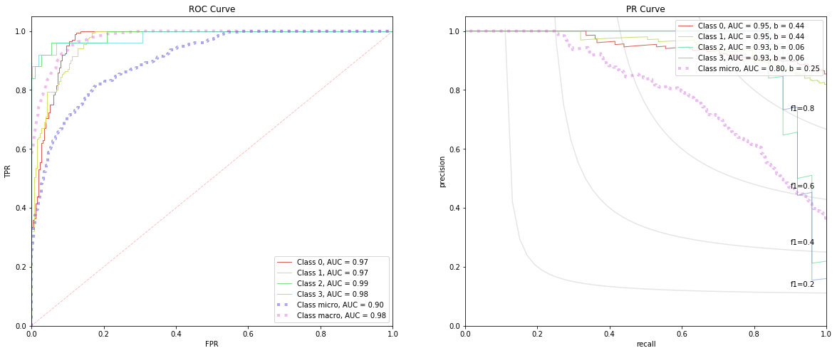
4.2.1. Training
[6]:
tpr, fpr, roc_auc, roc_keys = get_roc_stats(R)
precision, recall, average_precision, baselines, pr_keys = get_pr_stats(R)

fig, ax = plt.subplots(1, 2, figsize=(20, 8))
plot_rocs(tpr, fpr, roc_auc, roc_keys, ax[0])
plot_prs(precision, recall, average_precision, baselines, pr_keys, ax[1])
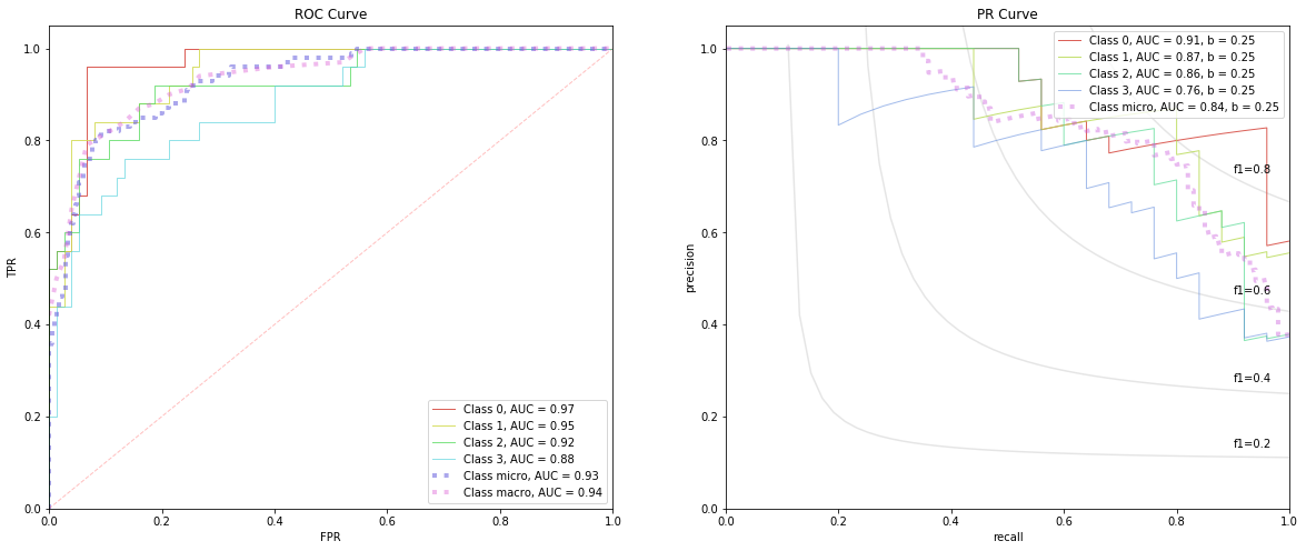
4.2.2. Testing
[7]:
tpr, fpr, roc_auc, roc_keys = get_roc_stats(E)
precision, recall, average_precision, baselines, pr_keys = get_pr_stats(E)

fig, ax = plt.subplots(1, 2, figsize=(20, 8))
plot_rocs(tpr, fpr, roc_auc, roc_keys, ax[0])
plot_prs(precision, recall, average_precision, baselines, pr_keys, ax[1])
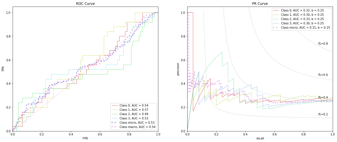
4.2.3. Validation
These are the curves that matter most as the validation data was never seen by the Inception model. Note how the AUC-ROC across all classes are no better than guess (very close to 0.5). Even the micro and macro AUC curves are aligned with the diagonal baseline. The AUC-PR curves are better than the corresponding baseline curves (except for Class 3), but still not that great.
[8]:
tpr, fpr, roc_auc, roc_keys = get_roc_stats(V)
precision, recall, average_precision, baselines, pr_keys = get_pr_stats(V)

fig, ax = plt.subplots(1, 2, figsize=(20, 8))
plot_rocs(tpr, fpr, roc_auc, roc_keys, ax[0])
plot_prs(precision, recall, average_precision, baselines, pr_keys, ax[1])