2. Pricing Elasticity of Demand Modeling
Pricing Elasticity of Demand (PED) is a measure of how responsive demand (or quantity sold) is to price change. When demand (y-axis) is plotted against price (x-axis), a demand curve is drawn. From the demand curve, we can compute the PED using pairs of points or at a particular point. Typically, elasticity changes along every point (or between every pair of points) on the demand curve. When we assume that elasticity remains constant along the demand curve, we can use regression techniques to estimate the constant elasticity. Let’s take a look to see how regression is used to estimate the constant elasticity.
2.1. Load data
This data is taken from Kaggle.
[1]:
import pandas as pd
import numpy as np

def get_text(r):
    product_category_name = r['product_category_name']


df = pd.read_csv('./data/retail_price.csv') \
    .assign(
        month_year=lambda d: pd.to_datetime(d['month_year']),
        year=lambda d: d['month_year'].dt.year,
        month=lambda d: d['month_year'].dt.month,
        weekend=lambda d: d['weekday'].apply(lambda x: 1 if x >= 5 else 0),
        text=lambda d: d['product_category_name'].apply(lambda s: ' '.join(s.split('_')))
    )
df.shape
[1]:
(676, 31)
[2]:
df.info()
<class 'pandas.core.frame.DataFrame'>
RangeIndex: 676 entries, 0 to 675
Data columns (total 31 columns):
 #   Column                      Non-Null Count  Dtype
---  ------                      --------------  -----
 0   product_id                  676 non-null    object
 1   product_category_name       676 non-null    object
 2   month_year                  676 non-null    datetime64[ns]
 3   qty                         676 non-null    int64
 4   total_price                 676 non-null    float64
 5   freight_price               676 non-null    float64
 6   unit_price                  676 non-null    float64
 7   product_name_lenght         676 non-null    int64
 8   product_description_lenght  676 non-null    int64
 9   product_photos_qty          676 non-null    int64
 10  product_weight_g            676 non-null    int64
 11  product_score               676 non-null    float64
 12  customers                   676 non-null    int64
 13  weekday                     676 non-null    int64
 14  weekend                     676 non-null    int64
 15  holiday                     676 non-null    int64
 16  month                       676 non-null    int64
 17  year                        676 non-null    int64
 18  s                           676 non-null    float64
 19  volume                      676 non-null    int64
 20  comp_1                      676 non-null    float64
 21  ps1                         676 non-null    float64
 22  fp1                         676 non-null    float64
 23  comp_2                      676 non-null    float64
 24  ps2                         676 non-null    float64
 25  fp2                         676 non-null    float64
 26  comp_3                      676 non-null    float64
 27  ps3                         676 non-null    float64
 28  fp3                         676 non-null    float64
 29  lag_price                   676 non-null    float64
 30  text                        676 non-null    object
dtypes: datetime64[ns](1), float64(15), int64(12), object(3)
memory usage: 163.8+ KB
2.2. Visualize pricing elasticity of demand
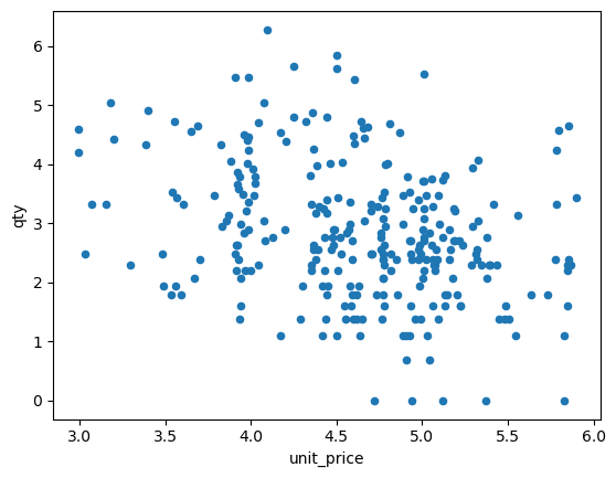
There’s already a lot of exploratory data analysis (EDA) and visualization on the data on Kaggle, and so we will not plot too much. Below, we are demand (quantity) versus price over all products. You can see that there tends to be a downward slope. Also note, we take the log of the demand and price.
[3]:
df[['unit_price', 'qty']] \
    .groupby(['unit_price']) \
    .sum() \
    .reset_index() \
    .assign(
        unit_price=lambda d: np.log(d['unit_price']),
        qty=lambda d: np.log(d['qty'])
    ) \
    .plot(kind='scatter', x='unit_price', y='qty')
[3]:
<Axes: xlabel='unit_price', ylabel='qty'>
2.3. Split into training/testing
It seems that there is data in 2017 for January and also in 2018 for January. Let’s use the 2017 data for training and the 2018 data for testing/validation.
[4]:
df['month_year'].value_counts().sort_index()
[4]:
2017-01-01     2
2017-01-02     9
2017-01-03    13
2017-01-04    15
2017-01-05    20
2017-01-06    25
2017-01-07    33
2017-01-08    37
2017-01-09    36
2017-01-10    43
2017-01-11    44
2017-01-12    44
2018-01-01    48
2018-01-02    49
2018-01-03    50
2018-01-04    48
2018-01-05    40
2018-01-06    42
2018-01-07    40
2018-01-08    38
Name: month_year, dtype: int64
[5]:
df_tr = df[df['month_year'] <= '2017-12-31']
df_te = df[df['month_year'] >= '2018-01-01']

df_tr.shape, df_te.shape
[5]:
((321, 31), (355, 31))
2.4. Simple log-log model
An easy way to model the relationship between price and quantity is using log-log regression. Note that the coefficient associated with price is the estimated constant elasticity.
\(\log{Q} \sim \log{P}\)
[6]:
Xy_tr = df_tr.groupby(['unit_price']) \
    .agg(qty_sum=pd.NamedAgg(column='qty', aggfunc='sum')) \
    .assign(qty_sum=lambda d: np.log(d['qty_sum'])) \
    .reset_index() \
    .assign(unit_price=lambda d: np.log(d['unit_price']))

Xy_te = df_te.groupby(['unit_price']) \
    .agg(qty_sum=pd.NamedAgg(column='qty', aggfunc='sum')) \
    .assign(qty_sum=lambda d: np.log(d['qty_sum'])) \
    .reset_index() \
    .assign(unit_price=lambda d: np.log(d['unit_price']))

X_tr = Xy_tr[['unit_price']]
X_te = Xy_te[['unit_price']]

y_tr = Xy_tr['qty_sum']
y_te = Xy_te['qty_sum']

X_tr.shape, X_te.shape, y_tr.shape, y_te.shape
[6]:
((128, 1), (181, 1), (128,), (181,))
Since we want to have fun and suspect that quantity and price may have linear or non-linear relationships, we will try out a few regression models.
[7]:
from sklearn.linear_model import LinearRegression
from sklearn.ensemble import RandomForestRegressor
from lightgbm import LGBMRegressor
from sklearn.metrics import mean_absolute_error

def get_performance(y_tr, z_tr, y_te, z_te):
    y_tr = np.exp(y_tr)
    z_tr = np.exp(z_tr)

    y_te = np.exp(y_te)
    z_te = np.exp(z_te)

    mae_tr = mean_absolute_error(y_tr, z_tr)
    mae_te = mean_absolute_error(y_te, z_te)

    mape_tr = np.mean(np.abs(y_tr - z_tr) / y_tr)
    mape_te = np.mean(np.abs(y_te - z_te) / y_te)

    wmape_tr = np.abs(y_tr - z_tr).sum() / y_tr.sum()
    wmape_te = np.abs(y_te - z_te).sum() / y_te.sum()

    s = pd.Series([
        mae_tr,
        mae_te,
        mape_tr,
        mape_te,
        wmape_tr,
        wmape_te,
        mae_tr / (y_tr.max() - y_tr.min()),
        mae_te / (y_te.max() - y_te.min()),
        mae_tr / y_tr.std(),
        mae_te / y_te.std(),
        mae_tr / y_tr.mean(),
        mae_te / y_te.mean()
    ], index=['mae_tr', 'mae_te',
              'mape_tr', 'mape_te',
              'wmape_tr', 'wmape_te',
              'range_mae_tr', 'range_mae_te',
              'std_mae_tr', 'std_mae_te',
              'mean_mae_tr', 'mean_mae_te'])

    return s

def get_performance_summary(models):
    for m in models:
        m.fit(X_tr, y_tr)

    df = pd.DataFrame([get_performance(y_tr, m.predict(X_tr), y_te, m.predict(X_te))
                  for m in models], index=['OLS', 'RF', 'GBT'])
    return df

loglog_models = [
    LinearRegression(),
    RandomForestRegressor(n_jobs=-1, random_state=37, n_estimators=25),
    LGBMRegressor(n_jobs=-1, random_state=37, num_leaves=10, n_estimators=50, max_depth=2)
]

get_performance_summary(loglog_models)
[7]:
| mae_tr | mae_te | mape_tr | mape_te | wmape_tr | wmape_te | range_mae_tr | range_mae_te | std_mae_tr | std_mae_te | mean_mae_tr | mean_mae_te | |
|---|---|---|---|---|---|---|---|---|---|---|---|---|
| OLS | 24.973284 | 21.790472 | 1.452983 | 1.164152 | 0.735184 | 0.723551 | 0.046679 | 0.076998 | 0.392888 | 0.509473 | 0.735184 | 0.723551 |
| RF | 12.091052 | 31.956025 | 0.449581 | 2.286806 | 0.355946 | 1.061097 | 0.022600 | 0.112919 | 0.190221 | 0.747149 | 0.355946 | 1.061097 |
| GBT | 24.513070 | 22.900274 | 1.366331 | 1.335325 | 0.721636 | 0.760402 | 0.045819 | 0.080920 | 0.385648 | 0.535421 | 0.721636 | 0.760402 |
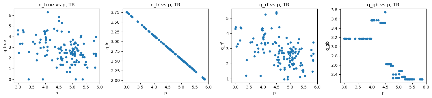
GBT seems to have the lowest validated MAE at 22.9.
[8]:
loglog_tr = pd.DataFrame({
    'p': X_tr['unit_price'].values,
    'q_true': y_tr.values,
    'q_lr': loglog_models[0].predict(X_tr),
    'q_rf': loglog_models[1].predict(X_tr),
    'q_gb': loglog_models[2].predict(X_tr)
})

loglog_te = pd.DataFrame({
    'p': X_te['unit_price'].values,
    'q_true': y_te.values,
    'q_lr': loglog_models[0].predict(X_te),
    'q_rf': loglog_models[1].predict(X_te),
    'q_gb': loglog_models[2].predict(X_te)
})
[9]:
import matplotlib.pyplot as plt

def do_scatter(df, title_suffix, p_field='p', q_fields=['q_true', 'q_lr', 'q_rf', 'q_gb']):
    fig, axes = plt.subplots(1, 4, figsize=(15, 3.5))

    for q_field, ax in zip(q_fields, np.ravel(axes)):
        df.plot(
            kind='scatter',
            x=p_field,
            y=q_field,
            ax=ax,
            title=f'{q_field} vs {p_field}, {title_suffix}'
        )

    fig.tight_layout()

def do_scatter_overlay(df_tr, df_te, p_field='p', q_fields=['q_true', 'q_lr', 'q_rf', 'q_gb']):
    fig, axes = plt.subplots(1, 4, figsize=(15, 3.5))

    for q_field, ax in zip(q_fields, np.ravel(axes)):
        df_tr.plot(kind='scatter', x=p_field, y=q_field, ax=ax, color='r', label='tr')
        df_te.plot(kind='scatter', x=p_field, y=q_field, ax=ax, color='b', label='te')
        ax.set_title(f'{q_field} vs {p_field}')

    fig.tight_layout()
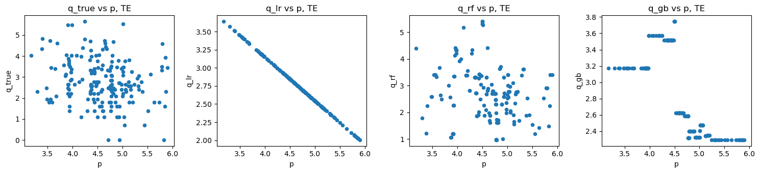
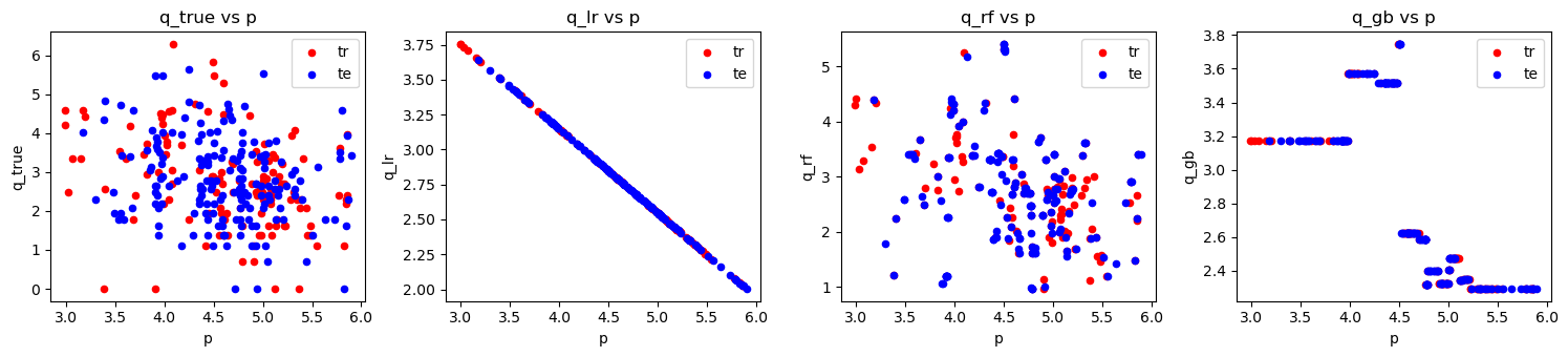
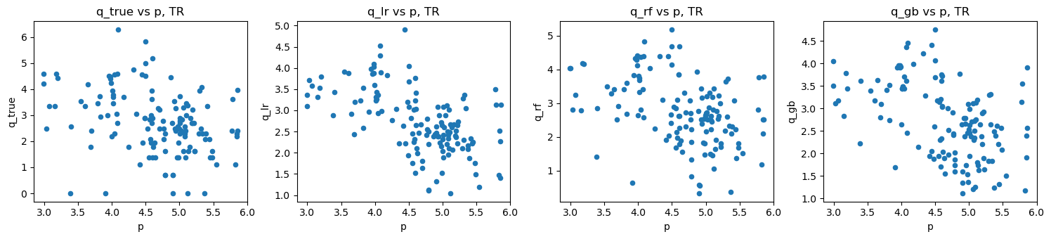
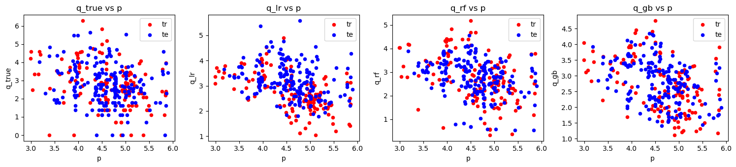
[10]:
do_scatter(loglog_tr, 'TR')
do_scatter(loglog_te, 'TE')
do_scatter_overlay(loglog_tr, loglog_te)
2.5. Log-log model with features
In the log-log model with features, we’ll add additional features to see if it helps in modeling and the models’ performances.
\(\log{Q} \sim \log{P} + X_1 + X_2 + \ldots + X_n\)
[11]:
def get_Xy(df):
    a = df.groupby(['product_category_name', 'unit_price']) \
        .agg(qty_sum=pd.NamedAgg(column='qty', aggfunc='sum')) \
        .assign(qty_sum=lambda d: np.log(d['qty_sum'])) \
        .rename(columns={'qty_sum': 'quantity'})

    b = df.groupby(['product_category_name', 'unit_price']) \
        .agg(
            freight_price=pd.NamedAgg(column='freight_price', aggfunc='mean'),
            product_score=pd.NamedAgg(column='product_score', aggfunc='mean'),
            weekday=pd.NamedAgg(column='weekday', aggfunc='mean'),
            holiday=pd.NamedAgg(column='holiday', aggfunc='mean'),
            customers=pd.NamedAgg(column='customers', aggfunc='mean'),
            volume=pd.NamedAgg(column='volume', aggfunc='mean'),
            s=pd.NamedAgg(column='s', aggfunc='mean'),
            comp_1=pd.NamedAgg(column='comp_1', aggfunc='mean'),
            ps1=pd.NamedAgg(column='ps1', aggfunc='mean'),
            fp1=pd.NamedAgg(column='fp1', aggfunc='mean'),
            comp_2=pd.NamedAgg(column='comp_2', aggfunc='mean'),
            ps2=pd.NamedAgg(column='ps2', aggfunc='mean'),
            fp2=pd.NamedAgg(column='fp2', aggfunc='mean'),
            comp_3=pd.NamedAgg(column='comp_3', aggfunc='mean'),
            ps3=pd.NamedAgg(column='ps3', aggfunc='mean'),
            fp3=pd.NamedAgg(column='fp3', aggfunc='mean'),
            lag_price=pd.NamedAgg(column='lag_price', aggfunc='mean')
        )

    Xy = a \
        .join(b, how='left') \
        .reset_index() \
        .assign(unit_price=lambda d: np.log(d['unit_price']))

    c = pd.get_dummies(Xy[['product_category_name']]).iloc[:,1:]

    Xy = Xy.join(c, how='left').drop(columns=['product_category_name'])

    X = Xy[Xy.columns.drop(['quantity'])]
    y = Xy['quantity']

    return X, y

X_tr, y_tr = get_Xy(df_tr)
X_te, y_te = get_Xy(df_te)

X_tr.shape, X_te.shape, y_tr.shape, y_te.shape
[11]:
((133, 26), (188, 26), (133,), (188,))
[12]:
loglog_plus_models = [
    LinearRegression(),
    RandomForestRegressor(n_jobs=-1, random_state=37, n_estimators=25),
    LGBMRegressor(n_jobs=-1, random_state=37, num_leaves=10, n_estimators=50, max_depth=2)
]

get_performance_summary(loglog_plus_models)
[12]:
| mae_tr | mae_te | mape_tr | mape_te | wmape_tr | wmape_te | range_mae_tr | range_mae_te | std_mae_tr | std_mae_te | mean_mae_tr | mean_mae_te | |
|---|---|---|---|---|---|---|---|---|---|---|---|---|
| OLS | 21.592945 | 28.363898 | 1.090862 | 2.246045 | 0.660502 | 0.978245 | 0.040361 | 0.100226 | 0.357261 | 0.677601 | 0.660502 | 0.978245 |
| RF | 10.259959 | 20.777510 | 0.281573 | 1.100575 | 0.313840 | 0.716597 | 0.019177 | 0.073419 | 0.169754 | 0.496366 | 0.313840 | 0.716597 |
| GBT | 15.886894 | 19.211437 | 0.611473 | 1.051234 | 0.485961 | 0.662585 | 0.029695 | 0.067885 | 0.262853 | 0.458953 | 0.485961 | 0.662585 |
GBT seems to have the lowest validated MAE at 19.2.
[13]:
loglog_plus_tr = pd.DataFrame({
    'p': X_tr['unit_price'].values,
    'q_true': y_tr.values,
    'q_lr': loglog_plus_models[0].predict(X_tr),
    'q_rf': loglog_plus_models[1].predict(X_tr),
    'q_gb': loglog_plus_models[2].predict(X_tr)
})

loglog_plus_te = pd.DataFrame({
    'p': X_te['unit_price'].values,
    'q_true': y_te.values,
    'q_lr': loglog_plus_models[0].predict(X_te),
    'q_rf': loglog_plus_models[1].predict(X_te),
    'q_gb': loglog_plus_models[2].predict(X_te)
})
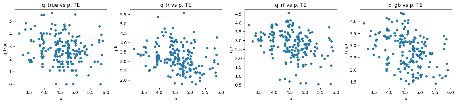
[14]:
do_scatter(loglog_plus_tr, 'TR')
do_scatter(loglog_plus_te, 'TE')
do_scatter_overlay(loglog_plus_tr, loglog_plus_te)
2.6. MERF model
The Mixed-Effect Random Forest (MERF) model uses a non-linear model to model the fixed effects but leaves the random effects as linear interaction terms.
\(y_i = f(X_i) + Z_i u_i + e_i\)
To use the MERF model, install it from git as follows.
pip install git+https://github.com/manifoldai/merf.git
[15]:
p2i = {c: i for i, c in enumerate(list(df['product_category_name'].unique()))}
i2p = {v: k for k, v in p2i.items()}
[16]:
def get_Xy(df):
    a = df.groupby(['product_id', 'product_category_name', 'unit_price']) \
        .agg(
            qty_sum=pd.NamedAgg(column='qty', aggfunc='sum'),
            freight_price=pd.NamedAgg(column='freight_price', aggfunc='mean'),
            product_score=pd.NamedAgg(column='product_score', aggfunc='mean'),
            comp_1=pd.NamedAgg(column='comp_1', aggfunc='mean'),
            ps1=pd.NamedAgg(column='ps1', aggfunc='mean'),
            fp1=pd.NamedAgg(column='fp1', aggfunc='mean'),
            comp_2=pd.NamedAgg(column='comp_2', aggfunc='mean'),
            ps2=pd.NamedAgg(column='ps2', aggfunc='mean'),
            fp2=pd.NamedAgg(column='fp2', aggfunc='mean'),
            comp_3=pd.NamedAgg(column='comp_3', aggfunc='mean'),
            ps3=pd.NamedAgg(column='ps3', aggfunc='mean'),
            fp3=pd.NamedAgg(column='fp3', aggfunc='mean'),
            lag_price=pd.NamedAgg(column='lag_price', aggfunc='mean')
        ) \
        .assign(
            qty_sum=lambda d: np.log(d['qty_sum'])
        ) \
        .rename(columns={'qty_sum': 'quantity'}) \
        .reset_index() \
        .drop(columns=['product_id']) \
        .set_index(['product_category_name', 'unit_price'])

    b = df.groupby(['product_category_name', 'unit_price']) \
        .agg(
            weekday=pd.NamedAgg(column='weekday', aggfunc='mean'),
            holiday=pd.NamedAgg(column='holiday', aggfunc='mean'),
            customers=pd.NamedAgg(column='customers', aggfunc='mean'),
            volume=pd.NamedAgg(column='volume', aggfunc='mean'),
            s=pd.NamedAgg(column='s', aggfunc='mean')
        )

    Xy = a \
        .join(b, how='inner') \
        .reset_index() \
        .assign(unit_price=lambda d: np.log(d['unit_price']))

    Xy = Xy.assign(product_category_name=lambda d: d['product_category_name'].map(p2i))

    X = Xy[Xy.columns.drop(['quantity', 'product_category_name', 'weekday', 'holiday', 'customers', 'volume', 's'])]
    Z = Xy[['weekday', 'holiday', 'customers', 's', 'lag_price']]
    C = Xy['product_category_name']
    y = Xy['quantity']

    return X, Z, C, y

X_tr, Z_tr, C_tr, y_tr = get_Xy(df_tr)
X_te, Z_te, C_te, y_te = get_Xy(df_te)
[17]:
X_tr.shape, Z_tr.shape, C_tr.shape, y_tr.shape
[17]:
((148, 13), (148, 5), (148,), (148,))
[18]:
X_te.shape, Z_te.shape, C_te.shape, y_te.shape
[18]:
((208, 13), (208, 5), (208,), (208,))
[19]:
from merf import MERF

merf = MERF(
    fixed_effects_model=LGBMRegressor(n_jobs=-1, random_state=37, num_leaves=10, n_estimators=25, max_depth=2),
    max_iterations=30
)
merf.fit(X_tr, Z_tr, C_tr, y_tr)
get_performance(y_tr, merf.predict(X_tr, Z_tr, C_tr), y_te, merf.predict(X_te, Z_te, C_te))
INFO     [merf.py:307] Training GLL is -101.1968163425363 at iteration 1.
INFO     [merf.py:307] Training GLL is -171.16405780723312 at iteration 2.
INFO     [merf.py:307] Training GLL is -212.75117155142982 at iteration 3.
INFO     [merf.py:307] Training GLL is -237.3949966765289 at iteration 4.
INFO     [merf.py:307] Training GLL is -251.62779481924196 at iteration 5.
INFO     [merf.py:307] Training GLL is -261.7722548752886 at iteration 6.
INFO     [merf.py:307] Training GLL is -270.91408548631705 at iteration 7.
INFO     [merf.py:307] Training GLL is -277.8358575135619 at iteration 8.
INFO     [merf.py:307] Training GLL is -284.2161675842258 at iteration 9.
INFO     [merf.py:307] Training GLL is -291.0438736305228 at iteration 10.
INFO     [merf.py:307] Training GLL is -296.86277233482656 at iteration 11.
INFO     [merf.py:307] Training GLL is -301.2918249236685 at iteration 12.
INFO     [merf.py:307] Training GLL is -309.2639355840515 at iteration 13.
INFO     [merf.py:307] Training GLL is -313.2097808051912 at iteration 14.
INFO     [merf.py:307] Training GLL is -317.2383961719355 at iteration 15.
INFO     [merf.py:307] Training GLL is -321.7435059133349 at iteration 16.
INFO     [merf.py:307] Training GLL is -325.2538612240947 at iteration 17.
INFO     [merf.py:307] Training GLL is -328.3921568512495 at iteration 18.
INFO     [merf.py:307] Training GLL is -331.5095703868812 at iteration 19.
INFO     [merf.py:307] Training GLL is -335.3589905785209 at iteration 20.
INFO     [merf.py:307] Training GLL is -338.9548103244854 at iteration 21.
INFO     [merf.py:307] Training GLL is -342.3731168294115 at iteration 22.
INFO     [merf.py:307] Training GLL is -345.4442477917209 at iteration 23.
INFO     [merf.py:307] Training GLL is -348.75818816407207 at iteration 24.
INFO     [merf.py:307] Training GLL is -352.5510448500377 at iteration 25.
INFO     [merf.py:307] Training GLL is -355.102251919231 at iteration 26.
INFO     [merf.py:307] Training GLL is -357.6226061099023 at iteration 27.
INFO     [merf.py:307] Training GLL is -358.64542456205777 at iteration 28.
INFO     [merf.py:307] Training GLL is -361.5995433713272 at iteration 29.
INFO     [merf.py:307] Training GLL is -362.07091949111447 at iteration 30.
[19]:
mae_tr          15.590045
mae_te          18.394509
mape_tr          0.750941
mape_te          1.331177
wmape_tr         0.530664
wmape_te         0.701900
range_mae_tr     0.045853
range_mae_te     0.064998
std_mae_tr       0.388801
std_mae_te       0.529736
mean_mae_tr      0.530664
mean_mae_te      0.701900
dtype: float64
We get a slight improvement with the MAE at 18.4. So far, the MAEs for the different models are as follows.
Log-log MAE: 22.9
Log-log + Features MAE: 19.2
MERF MAE: 18.4
Below are the feature importances for the fixed effects variables.
[20]:
pd.Series(merf.fe_model.feature_importances_, X_tr.columns) \
    .sort_values(ascending=False)
[20]:
unit_price       25
freight_price    11
fp1               9
fp2               7
comp_3            7
ps3               4
ps2               3
fp3               2
lag_price         2
product_score     0
comp_1            0
ps1               0
comp_2            0
dtype: int32
Below are the coefficients for the random effects by the grouping variable (which are the product categories).
[21]:
merf.trained_b.sort_index() \
    .rename(columns={0: 'weekday', 1: 'holiday', 2: 'customers', 3: 'volume', 4: 's', 5: 'lag_price'}) \
    .T \
    .rename(columns=i2p).T
[21]:
| weekday | holiday | customers | volume | s | |
|---|---|---|---|---|---|
| bed_bath_table | -0.007945 | -0.186044 | 0.000864 | 0.035106 | -0.002121 |
| garden_tools | -0.030065 | -0.062398 | 0.001513 | 0.052798 | -0.004259 |
| consoles_games | -0.004937 | -0.007303 | 0.000203 | 0.009453 | -0.000838 |
| health_beauty | 0.016584 | -0.038887 | -0.000543 | -0.018656 | 0.001668 |
| cool_stuff | 0.003853 | 0.133319 | 0.000107 | -0.026230 | 0.001764 |
| perfumery | -0.003835 | -0.027635 | 0.000262 | 0.009871 | -0.000816 |
| computers_accessories | -0.028299 | 0.319809 | 0.001429 | -0.003708 | -0.001072 |
| watches_gifts | -0.030244 | 0.035122 | 0.002325 | 0.034548 | -0.002885 |
| furniture_decor | 0.007239 | 0.042501 | -0.000677 | -0.013164 | 0.000763 |
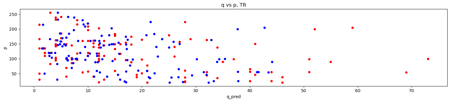
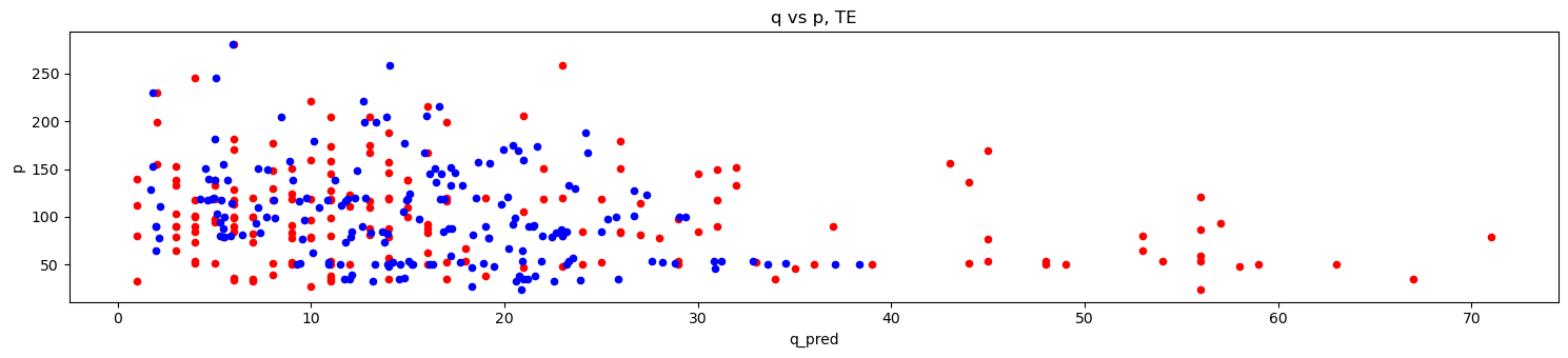
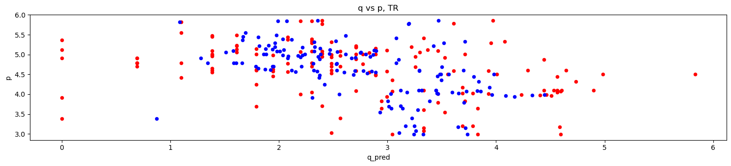
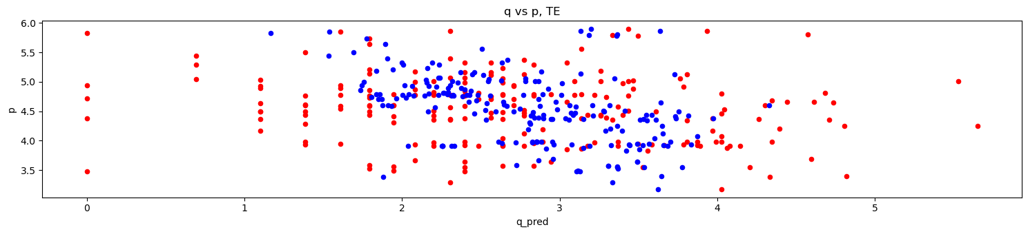
[22]:
def do_merf_scatter(df, title_suffix):
    fig, ax = plt.subplots(figsize=(15, 3.5))

    df.plot(kind='scatter', x='q_true', y='p', ax=ax, color='r')
    df.plot(kind='scatter', x='q_pred', y='p', ax=ax, color='b')

    ax.set_title(f'q vs p, {title_suffix}')

    fig.tight_layout()
[23]:
do_merf_scatter(pd.DataFrame({
    'p': X_tr['unit_price'].values,
    'q_true': y_tr.values,
    'q_pred': merf.predict(X_tr, Z_tr, C_tr)
}), 'TR')

do_merf_scatter(pd.DataFrame({
    'p': X_te['unit_price'].values,
    'q_true': y_te.values,
    'q_pred': merf.predict(X_te, Z_te, C_te)
}), 'TE')
2.7. MERF + features
Let’s make the MERF models more sophisticated by adding in more fixed and random effects.
[24]:
p2i = {c: i for i, c in enumerate(list(df['product_id'].unique()))}
i2p = {v: k for k, v in p2i.items()}
[25]:
c2i = {c: i for i, c in enumerate(list(df['product_category_name'].unique()))}
i2c = {v: k for k, v in p2i.items()}
[26]:
def get_Xy(df):
    a = df.groupby(['product_id', 'product_category_name', 'unit_price']) \
        .agg(
            qty_sum=pd.NamedAgg(column='qty', aggfunc='sum'),
            freight_price=pd.NamedAgg(column='freight_price', aggfunc='mean'),
            product_score=pd.NamedAgg(column='product_score', aggfunc='mean'),
            comp_1=pd.NamedAgg(column='comp_1', aggfunc='mean'),
            ps1=pd.NamedAgg(column='ps1', aggfunc='mean'),
            fp1=pd.NamedAgg(column='fp1', aggfunc='mean'),
            comp_2=pd.NamedAgg(column='comp_2', aggfunc='mean'),
            ps2=pd.NamedAgg(column='ps2', aggfunc='mean'),
            fp2=pd.NamedAgg(column='fp2', aggfunc='mean'),
            comp_3=pd.NamedAgg(column='comp_3', aggfunc='mean'),
            ps3=pd.NamedAgg(column='ps3', aggfunc='mean'),
            fp3=pd.NamedAgg(column='fp3', aggfunc='mean'),
            lag_price=pd.NamedAgg(column='lag_price', aggfunc='mean')
        ) \
        .assign(
            qty_sum=lambda d: np.log(d['qty_sum'])
        ) \
        .rename(columns={'qty_sum': 'quantity'}) \
        .reset_index() \
        .assign(
            bed1=lambda d: np.where(d['product_id']=='bed1', 1, 0),
            garden5=lambda d: np.where(d['product_id']=='garden5', 1, 0),
            consoles1=lambda d: np.where(d['product_id']=='consoles1', 1, 0),
            garden7=lambda d: np.where(d['product_id']=='garden7', 1, 0),
            health9=lambda d: np.where(d['product_id']=='health9', 1, 0),
            cool4=lambda d: np.where(d['product_id']=='cool4', 1, 0),
            health3=lambda d: np.where(d['product_id']=='health3', 1, 0),
            perfumery1=lambda d: np.where(d['product_id']=='perfumery1', 1, 0),
            cool5=lambda d: np.where(d['product_id']=='cool5', 1, 0),
            health8=lambda d: np.where(d['product_id']=='health8', 1, 0),
            garden4=lambda d: np.where(d['product_id']=='garden4', 1, 0),
            computers5=lambda d: np.where(d['product_id']=='computers5', 1, 0),
            garden10=lambda d: np.where(d['product_id']=='garden10', 1, 0),
            computers6=lambda d: np.where(d['product_id']=='computers6', 1, 0),
            health6=lambda d: np.where(d['product_id']=='health6', 1, 0),
            garden6=lambda d: np.where(d['product_id']=='garden6', 1, 0),
            health10=lambda d: np.where(d['product_id']=='health10', 1, 0),
            watches2=lambda d: np.where(d['product_id']=='watches2', 1, 0),
            health1=lambda d: np.where(d['product_id']=='health1', 1, 0),
            garden8=lambda d: np.where(d['product_id']=='garden8', 1, 0),
            garden9=lambda d: np.where(d['product_id']=='garden9', 1, 0),
            watches6=lambda d: np.where(d['product_id']=='watches6', 1, 0),
            cool3=lambda d: np.where(d['product_id']=='cool3', 1, 0),
            perfumery2=lambda d: np.where(d['product_id']=='perfumery2', 1, 0),
            cool2=lambda d: np.where(d['product_id']=='cool2', 1, 0),
            computers1=lambda d: np.where(d['product_id']=='computers1', 1, 0),
            consoles2=lambda d: np.where(d['product_id']=='consoles2', 1, 0),
            health5=lambda d: np.where(d['product_id']=='health5', 1, 0),
            watches8=lambda d: np.where(d['product_id']=='watches8', 1, 0),
            furniture4=lambda d: np.where(d['product_id']=='furniture4', 1, 0),
            watches5=lambda d: np.where(d['product_id']=='watches5', 1, 0),
            health7=lambda d: np.where(d['product_id']=='health7', 1, 0),
            bed3=lambda d: np.where(d['product_id']=='bed3', 1, 0),
            garden3=lambda d: np.where(d['product_id']=='garden3', 1, 0),
            bed2=lambda d: np.where(d['product_id']=='bed2', 1, 0),
            furniture3=lambda d: np.where(d['product_id']=='furniture3', 1, 0),
            watches4=lambda d: np.where(d['product_id']=='watches4', 1, 0),
            watches3=lambda d: np.where(d['product_id']=='watches3', 1, 0),
            furniture2=lambda d: np.where(d['product_id']=='furniture2', 1, 0),
            garden2=lambda d: np.where(d['product_id']=='garden2', 1, 0),
            furniture1=lambda d: np.where(d['product_id']=='furniture1', 1, 0),
            health2=lambda d: np.where(d['product_id']=='health2', 1, 0),
            garden1=lambda d: np.where(d['product_id']=='garden1', 1, 0),
            cool1=lambda d: np.where(d['product_id']=='cool1', 1, 0),
            computers4=lambda d: np.where(d['product_id']=='computers4', 1, 0),
            watches7=lambda d: np.where(d['product_id']=='watches7', 1, 0),
            computers3=lambda d: np.where(d['product_id']=='computers3', 1, 0),
            health4=lambda d: np.where(d['product_id']=='health4', 1, 0),
            watches1=lambda d: np.where(d['product_id']=='watches1', 1, 0),
            computers2=lambda d: np.where(d['product_id']=='computers2', 1, 0),
            bed4=lambda d: np.where(d['product_id']=='bed4', 1, 0),
            bed5=lambda d: np.where(d['product_id']=='bed5', 1, 0)
        ) \
        .drop(columns=['product_id']) \
        .set_index(['product_category_name', 'unit_price'])

    b = df.groupby(['product_category_name', 'unit_price']) \
        .agg(
            weekday=pd.NamedAgg(column='weekday', aggfunc='mean'),
            holiday=pd.NamedAgg(column='holiday', aggfunc='mean'),
            customers=pd.NamedAgg(column='customers', aggfunc='mean'),
            volume=pd.NamedAgg(column='volume', aggfunc='mean'),
            s=pd.NamedAgg(column='s', aggfunc='mean')
        ) \
        .reset_index() \
        .assign(
            bed_bath_table=lambda d: np.where(d['product_category_name']=='bed_bath_table', 1, 0),
            garden_tools=lambda d: np.where(d['product_category_name']=='garden_tools', 1, 0),
            consoles_games=lambda d: np.where(d['product_category_name']=='consoles_games', 1, 0),
            health_beauty=lambda d: np.where(d['product_category_name']=='health_beauty', 1, 0),
            cool_stuff=lambda d: np.where(d['product_category_name']=='cool_stuff', 1, 0),
            perfumery=lambda d: np.where(d['product_category_name']=='perfumery', 1, 0),
            computers_accessories=lambda d: np.where(d['product_category_name']=='computers_accessories', 1, 0),
            watches_gifts=lambda d: np.where(d['product_category_name']=='watches_gifts', 1, 0),
            furniture_decor=lambda d: np.where(d['product_category_name']=='furniture_decor', 1, 0)
        ) \
        .set_index(['product_category_name', 'unit_price'])

    Xy = a \
        .join(b, how='inner') \
        .reset_index() \
        .assign(unit_price=lambda d: np.log(d['unit_price']))

    Xy = Xy.assign(product_category_name=lambda d: d['product_category_name'].map(c2i)) \
        .query('unit_price < 5.7') \
        .query('quantity < 4.3')

    X = Xy[Xy.columns.drop(['quantity', 'product_category_name', 'bed_bath_table', 'garden_tools', 'consoles_games', 'health_beauty', 'cool_stuff', 'perfumery', 'computers_accessories', 'watches_gifts', 'furniture_decor', 'weekday', 'holiday', 'customers', 'volume', 's'])]
    Z = Xy[['bed_bath_table', 'garden_tools', 'consoles_games', 'health_beauty', 'cool_stuff', 'perfumery', 'computers_accessories', 'watches_gifts', 'furniture_decor', 'weekday', 'holiday', 'customers', 's']]
    C = Xy['product_category_name']
    y = Xy['quantity']

    return X, Z, C, y

X_tr, Z_tr, C_tr, y_tr = get_Xy(df_tr)
X_te, Z_te, C_te, y_te = get_Xy(df_te)
[27]:
X_tr.shape, Z_tr.shape, C_tr.shape, y_tr.shape
[27]:
((123, 65), (123, 13), (123,), (123,))
[28]:
X_te.shape, Z_te.shape, C_te.shape, y_te.shape
[28]:
((184, 65), (184, 13), (184,), (184,))
[29]:
merf = MERF(
    fixed_effects_model=LGBMRegressor(n_jobs=-1, random_state=37, num_leaves=500, n_estimators=5, max_depth=100),
    max_iterations=30
)
merf.fit(X_tr, Z_tr, C_tr, y_tr)
get_performance(y_tr, merf.predict(X_tr, Z_tr, C_tr), y_te, merf.predict(X_te, Z_te, C_te))
INFO     [merf.py:307] Training GLL is -88.13270721590854 at iteration 1.
INFO     [merf.py:307] Training GLL is -131.66918167831366 at iteration 2.
INFO     [merf.py:307] Training GLL is -158.3396085429746 at iteration 3.
INFO     [merf.py:307] Training GLL is -172.36626681950983 at iteration 4.
INFO     [merf.py:307] Training GLL is -183.273845220244 at iteration 5.
INFO     [merf.py:307] Training GLL is -195.50527698451978 at iteration 6.
INFO     [merf.py:307] Training GLL is -206.25905996127523 at iteration 7.
INFO     [merf.py:307] Training GLL is -216.38182995185898 at iteration 8.
INFO     [merf.py:307] Training GLL is -226.02365508411302 at iteration 9.
INFO     [merf.py:307] Training GLL is -235.22712598205717 at iteration 10.
INFO     [merf.py:307] Training GLL is -244.08248099738415 at iteration 11.
INFO     [merf.py:307] Training GLL is -252.6305118737953 at iteration 12.
INFO     [merf.py:307] Training GLL is -260.89381991319885 at iteration 13.
INFO     [merf.py:307] Training GLL is -268.9004674811783 at iteration 14.
INFO     [merf.py:307] Training GLL is -276.6759567855772 at iteration 15.
INFO     [merf.py:307] Training GLL is -284.2689734523188 at iteration 16.
INFO     [merf.py:307] Training GLL is -291.6957739036444 at iteration 17.
INFO     [merf.py:307] Training GLL is -300.27162761932044 at iteration 18.
INFO     [merf.py:307] Training GLL is -307.3709908011281 at iteration 19.
INFO     [merf.py:307] Training GLL is -314.25093506142235 at iteration 20.
INFO     [merf.py:307] Training GLL is -320.95384324169385 at iteration 21.
INFO     [merf.py:307] Training GLL is -327.49634087153373 at iteration 22.
INFO     [merf.py:307] Training GLL is -334.8272808170837 at iteration 23.
INFO     [merf.py:307] Training GLL is -339.9610697921489 at iteration 24.
INFO     [merf.py:307] Training GLL is -347.1184754251438 at iteration 25.
INFO     [merf.py:307] Training GLL is -353.1474426017086 at iteration 26.
INFO     [merf.py:307] Training GLL is -358.9569538145549 at iteration 27.
INFO     [merf.py:307] Training GLL is -364.6142070424412 at iteration 28.
INFO     [merf.py:307] Training GLL is -370.1421471030787 at iteration 29.
INFO     [merf.py:307] Training GLL is -375.51542805296117 at iteration 30.
[29]:
mae_tr           7.865860
mae_te          12.273571
mape_tr          0.727956
mape_te          1.127332
wmape_tr         0.446264
wmape_te         0.663436
range_mae_tr     0.109248
range_mae_te     0.175337
std_mae_tr       0.506936
std_mae_te       0.772760
mean_mae_tr      0.446264
mean_mae_te      0.663436
dtype: float64
So far, the MAEs for the different models are as follows.
Log-log MAE: 22.9
Log-log + Features MAE: 19.2
MERF MAE: 18.4
MERF + Features MAE: 12.3
[30]:
gbm = LGBMRegressor(n_jobs=-1, random_state=37, num_leaves=10, n_estimators=50, max_depth=100)
gbm.fit(X_tr.join(Z_tr), y_tr)
[30]:
LGBMRegressor(max_depth=100, n_estimators=50, num_leaves=10, random_state=37)In a Jupyter environment, please rerun this cell to show the HTML representation or trust the notebook.
On GitHub, the HTML representation is unable to render, please try loading this page with nbviewer.org.
LGBMRegressor(max_depth=100, n_estimators=50, num_leaves=10, random_state=37)
[31]:
get_performance(y_tr, gbm.predict(X_tr.join(Z_tr)), y_te, gbm.predict(X_te.join(Z_te)))
[31]:
mae_tr           6.141472
mae_te          10.011228
mape_tr          0.483427
mape_te          1.043864
wmape_tr         0.348432
wmape_te         0.541147
range_mae_tr     0.085298
range_mae_te     0.143018
std_mae_tr       0.395804
std_mae_te       0.630320
mean_mae_tr      0.348432
mean_mae_te      0.541147
dtype: float64
So far, the MAEs for the different models are as follows.
Log-log MAE: 22.9
Log-log + Features MAE: 19.2
MERF MAE: 18.4
MERF + Features MAE: 12.3
MERF + Features (GB) MAE: 10.0
2.8. Random forest
Let’s just use a random forest regressor without any mixed modelling.
[32]:
rf = RandomForestRegressor(
    n_jobs=-1,
    random_state=37,
    n_estimators=500,
    criterion='absolute_error',
    bootstrap=True,
    warm_start=True,
    min_samples_split=5
)
rf.fit(X_tr.join(Z_tr), y_tr)

get_performance(y_tr, rf.predict(X_tr.join(Z_tr)), y_te, rf.predict(X_te.join(Z_te)))
[32]:
mae_tr           3.733740
mae_te          10.506863
mape_tr          0.264830
mape_te          0.974256
wmape_tr         0.211831
wmape_te         0.567939
range_mae_tr     0.051857
range_mae_te     0.150098
std_mae_tr       0.240631
std_mae_te       0.661526
mean_mae_tr      0.211831
mean_mae_te      0.567939
dtype: float64
So far, the MAEs for the different models are as follows.
Log-log MAE: 22.9
Log-log + Features MAE: 19.2
MERF MAE: 18.4
MERF + Features MAE: 12.3
MERF + Features (GB) MAE: 10.0
RF MAE: 10.5
[33]:
do_merf_scatter(pd.DataFrame({
    'p': np.exp(X_tr['unit_price'].values),
    'q_true': np.exp(y_tr.values),
    'q_pred': np.exp(rf.predict(X_tr.join(Z_tr)))
}), 'TR')

do_merf_scatter(pd.DataFrame({
    'p': np.exp(X_te['unit_price'].values),
    'q_true': np.exp(y_te.values),
    'q_pred': np.exp(rf.predict(X_te.join(Z_te)))
}), 'TE')