4. Schedule Risk Analysis Distributions

The following are some distributions commonly used in Schedule Risk Analysis (SRA).

• Triangular

• Beta

• Beta Rectangular

• Doubly-Truncated

• Log-Normal

• Weibull

In this notebook, we will create classes to represet each distribution. In general, the classes will store the parameters, and three methods are available.

• pdf to compute the probability of a sample, x

• cdf to compute the cummulative distribution within a range a (low end) and b (high end)

• rvs to sample from the distribution

Of particular interest is the rvs method, which may be used in Monte Carlo simulation in SRA. Metrics such as

• Criticality Index (CI): measures the probability that an activity is on the critical path

• Significance Index (SI): measures the relative importance of an activity

• Schedule Sensitivity Index (SSI): measures the relative imporance of an activity taking CI into account

• Cruciality Index (CRI): measures the correlation between the activity duration and total project duration

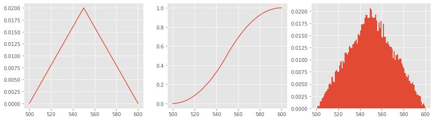
4.1. Triangular

The Triangular distribution is sometimes called a three-point estimate since it requires 3 parameters to create the distribution and the distribution’s probability density shape ends up looking like a triangle. The parameters are

• a minimum duration,

• m expected duration, and

• b maximum duration.

The probability density function (PDF) for the triangular distribution is as follows.

\(f(x) = \begin{cases} 0 & \text{for } x < a, \\ \frac{2(x-a)}{(b-a)(c-a)} & \text{for } a \le x < c, \\ \frac{2}{b-a} & \text{for } x = c, \\ \frac{2(b-x)}{(b-a)(b-c)} & \text{for } c < x \le b, \\ 0 & \text{for } b < x. \end{cases}\)

%matplotlib inline
import numpy as np
import random
import matplotlib.pyplot as plt
from numpy.random import uniform

random.seed(37)
np.random.seed(37)
plt.style.use('ggplot')

class Triangle(object):
    def __init__(self, a, m, b):
        self.a = a
        self.m = m
        self.b = b

    def pdf(self, x):
        a, m, b = self.a, self.m, self.b

        if b < x < a:
            return 0.0
        elif a <= x < m:
            return (2 * (x - a)) / ((b - a) * (m - a))
        elif x == m:
            return (2 / (b - a))
        elif m < x <= b:
            return (2 * (b - x)) / ((b - a) * (b - m))
        raise Exception(f'No conditions satisifed x={x}, {a}, {m}, {b}')

    def cdf(self):
        p = np.array([self.pdf(x) for x in range(a, b+1)])
        c = p.cumsum()
        return c

    def rvs(self, size=1):
        a, b = self.a, self.b

        o = {i:v for i, v in enumerate(range(a, b+1))}
        c = self.cdf()
        u = uniform(size=size)
        s = [o[np.argmax(c >= x)] for x in u]
        return np.array(s)

a, m, b = 500, 550, 600

d = Triangle(a, m, b)

p = [d.pdf(x) for x in range(a, b+1)]
c = d.cdf()
s = d.rvs(size=20000)

fig, ax = plt.subplots(1, 3, figsize=(15, 4))
_ = ax[0].plot(list(range(a, b+1)), p)
_ = ax[1].plot(list(range(a, b+1)), c)
_ = ax[2].hist(s, bins=list(range(a, b+1)), density=True)

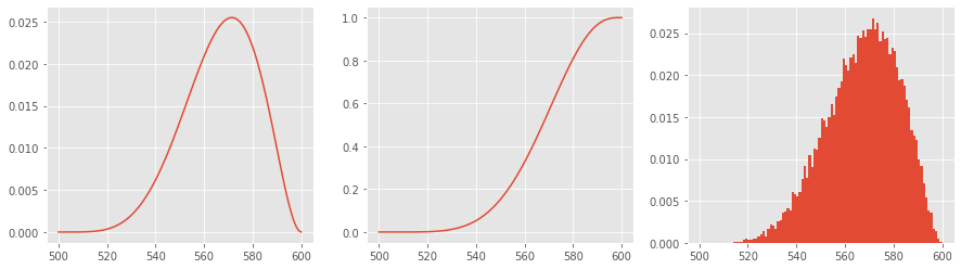
4.2. Beta

The Beta distribution is smoother and curved compared to the Triangular distribution. It is parameterized by the following.

• a minimum duration

• b maximum duration

• \(\theta_1\) shape parameter

• \(\theta_2\) shape parameter

Note that \(\theta_1\) and \(\theta_2\) are positive and modified to make the the distribution left (\(\theta_1 > \theta_2\)) or right skewed (\(\theta_1 < \theta_2\)). The PDF of the Beta distribution is defined as follows.

\(f(x) = \phi \frac{\Gamma(\theta_1 + \theta_2)}{\Gamma(\theta_1) \Gamma(\theta_2) (b - a)^{\theta_1 + \theta_2 - 1}}\)

from scipy.special import gamma

class Beta(object):
    def __init__(self, a, b, theta_1, theta_2):
        self.a = a
        self.b = b
        self.theta_1 = theta_1
        self.theta_2 = theta_2

    def pdf(self, x):
        a, b, theta_1, theta_2 = self.a, self.b, self.theta_1, self.theta_2

        p = gamma(theta_1 + theta_2)
        p = p / gamma(theta_1)
        p = p / gamma(theta_2)
        p = p / (b - a)**(theta_1 + theta_2 - 1)
        p = p * (x - a)**(theta_1 - 1)
        p = p * (b - x)**(theta_2 - 1)
        return p

    def cdf(self):
        p = np.array([self.pdf(x) for x in range(a, b+1)])
        c = p.cumsum()
        return c

    def rvs(self, size=1):
        a, b = self.a, self.b

        o = {i:v for i, v in enumerate(range(a, b+1))}
        c = self.cdf()
        u = uniform(size=size)
        s = [o[np.argmax(c >= x)] for x in u]
        return np.array(s)

a, b = 500, 600
theta_1, theta_2 = 6, 3

d = Beta(a, b, theta_1, theta_2)

p = [d.pdf(x) for x in range(a, b+1)]
c = d.cdf()
s = d.rvs(size=20000)

fig, ax = plt.subplots(1, 3, figsize=(15, 4))
_ = ax[0].plot(list(range(a, b+1)), p)
_ = ax[1].plot(list(range(a, b+1)), c)
_ = ax[2].hist(s, bins=list(range(a, b+1)), density=True)

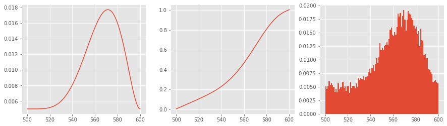
4.3. Beta Rectangular

The Beta Rectangular distribution is a mixture distribution of the Beta and Uniform distributions. It allows for an estimator’s judgement to vary between Beta and complete uncertainty (Uniform). The parameters for a Beta Rectangular distribution are as follows.

• a minimum duration

• b maximum duration

• \(\theta_1\) shape parameter

• \(\theta_2\) shape parameter

• \(\theta\) mixing parameter

Note that when \(\theta=1\), then the Beta distribution is recovered, and when \(\theta=0\), then the Uniform distribution is recovered. The parameter \(\theta\) is called the mixing parameter. The PDF of the Beta Rectangular is defined as follows.

\(f(x) = \phi \frac{\Gamma(\theta_1 + \theta_2)}{\Gamma(\theta_1) \Gamma(\theta_2) (b - a)^{\theta_1 + \theta_2 - 1}} + \frac{1 - \theta}{b - a}\)

class BetaRect(object):
    def __init__(self, a, b, theta_1, theta_2, theta):
        self.a = a
        self.b = b
        self.theta_1 = theta_1
        self.theta_2 = theta_2
        self.theta = theta

    def pdf(self, x):
        a, b = self.a, self.b
        theta_1, theta_2, theta = self.theta_1, self.theta_2, self.theta

        p = gamma(theta_1 + theta_2)
        p = p / gamma(theta_1)
        p = p / gamma(theta_2)
        p = p / (b - a)**(theta_1 + theta_2 - 1)
        p = p * (x - a)**(theta_1 - 1)
        p = p * (b - x)**(theta_2 - 1)
        p = p * theta
        p = p + ((1 - theta) / (b - a))
        return p

    def cdf(self):
        p = np.array([self.pdf(x) for x in range(a, b+1)])
        c = p.cumsum()
        return c

    def rvs(self, size=1):
        a, b = self.a, self.b

        o = {i:v for i, v in enumerate(range(a, b+1))}
        c = self.cdf()
        u = uniform(size=size)
        s = [o[np.argmax(c >= x)] for x in u]
        return np.array(s)

a, b = 500, 600
theta_1, theta_2 = 6, 3
theta = 0.5

d = BetaRect(a, b, theta_1, theta_2, theta)

p = [d.pdf(x) for x in range(a, b+1)]
c = d.cdf()
s = d.rvs(size=20000)

fig, ax = plt.subplots(1, 3, figsize=(15, 4))
_ = ax[0].plot(list(range(a, b+1)), p)
_ = ax[1].plot(list(range(a, b+1)), c)
_ = ax[2].hist(s, bins=list(range(a, b+1)), density=True)

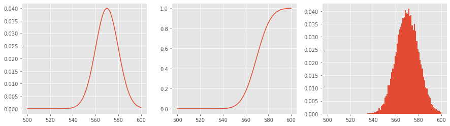
4.4. Doubly-truncated

Compared to the Beta distribution, the Doubly-truncated distribution emphasizes more on the mode. It is parameterized by the following.

• a minimum duration

• b maximum duration

• \(\mu\) mean

• \(\sigma\) standard deviation

The PDF of the Doubly-truncated distribution is defined as follows.

\(f(x)=\frac{\phi(\frac{x - \mu}{\sigma})}{\sigma( \Phi(\frac{b - \mu}{\sigma}) - \Phi(\frac{b - \mu}{\sigma}) )}\)

from scipy.stats import norm

class DoublyTruncated(object):
    def __init__(self, a, b, mu, sigma):
        self.a = a
        self.b = b
        self.mu = mu
        self.sigma = sigma

    def pdf(self, x):
        a, b = self.a, self.b
        mu, sigma = self.mu, self.sigma

        n = norm.pdf((x - mu) / sigma)
        d1 = norm.cdf((b - mu) / sigma)
        d2 = norm.cdf((a - mu) / sigma)
        d = sigma * (d1 - d2)
        p = n / d
        return p

    def cdf(self):
        p = np.array([self.pdf(x) for x in range(a, b+1)])
        c = p.cumsum()
        return c

    def rvs(self, size=1):
        a, b = self.a, self.b

        o = {i:v for i, v in enumerate(range(a, b+1))}
        c = self.cdf()
        u = uniform(size=size)
        s = [o[np.argmax(c >= x)] for x in u]
        return np.array(s)

a, b = 500, 600
mu, sigma = 570, 10

d = DoublyTruncated(a, b, mu, sigma)

p = [d.pdf(x) for x in range(a, b+1)]
c = d.cdf()
s = d.rvs(size=20000)

fig, ax = plt.subplots(1, 3, figsize=(15, 4))
_ = ax[0].plot(list(range(a, b+1)), p)
_ = ax[1].plot(list(range(a, b+1)), c)
_ = ax[2].hist(s, bins=list(range(a, b+1)), density=True)

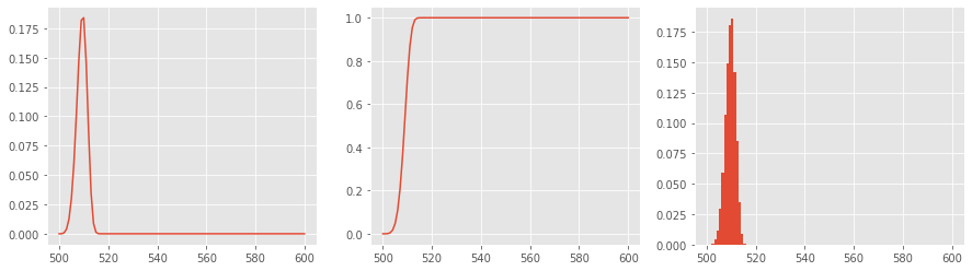
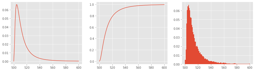
4.5. Log-normal

The Log-normal distribution is used in SRA when activities are right-skewed. This distribution has the following parameters.

• \(\mu\) mean

• \(\sigma\) standard deviation

The PDF of the Log-normal distribution is defined as follows.

\(f(x)=\frac{1}{x} \frac{1}{\sigma\sqrt{2\pi}} \exp\left( -\frac{(\ln x-\mu)^2}{2\sigma^2}\right)\)

from scipy.stats import lognorm

class LogNormal(object):
    def __init__(self, a, b, s, mu, sigma):
        self.a = a
        self.b = b
        self.s = s
        self.mu = mu
        self.sigma = sigma

    def pdf(self, x):
        s, mu, sigma = self.s, self.mu, self.sigma

        return lognorm.pdf(x, s, loc=mu, scale=sigma)

    def cdf(self):
        a, b = self.a, self.b

        p = np.array([self.pdf(x) for x in range(a, b+1)])
        c = p.cumsum()
        return c

    def rvs(self, size=1):
        a, b = self.a, self.b

        o = {i:v for i, v in enumerate(range(a, b+1))}
        c = self.cdf()
        u = uniform(size=size)
        s = [o[np.argmax(c >= x)] for x in u]
        return np.array(s)

a, b = 500, 600
mu, sigma, s = 500, 10, 0.9

d = LogNormal(a, b, s, mu, sigma)

p = [d.pdf(x) for x in range(a, b+1)]
c = d.cdf()
s = d.rvs(size=20000)

fig, ax = plt.subplots(1, 3, figsize=(15, 4))
_ = ax[0].plot(list(range(a, b+1)), p)
_ = ax[1].plot(list(range(a, b+1)), c)
_ = ax[2].hist(s, bins=list(range(a, b+1)), density=True)

4.6. Weibull

Compared to the Log-normal distribution, the Weibull distribution is used when activity durations are left-skewed. Its parameters are as follows.

• \(\mu\) mean

• \(\sigma\) standard deviation

The PDF of the Weibull is defined as follows.

\(f(x;\lambda,k) = \begin{cases} \frac{k}{\lambda}\left(\frac{x}{\lambda}\right)^{k-1}e^{-(x/\lambda)^{k}} & x\geq0 ,\\ 0 & x<0, \end{cases}\)

from scipy.stats import weibull_min

class Weibull(object):
    def __init__(self, a, b, s, mu, sigma):
        self.a = a
        self.b = b
        self.s = s
        self.mu = mu
        self.sigma = sigma

    def pdf(self, x):
        s, mu, sigma = self.s, self.mu, self.sigma

        return weibull_min.pdf(x, s, loc=mu, scale=sigma)

    def cdf(self):
        a, b = self.a, self.b

        p = np.array([self.pdf(x) for x in range(a, b+1)])
        c = p.cumsum()
        return c

    def rvs(self, size=1):
        a, b = self.a, self.b

        o = {i:v for i, v in enumerate(range(a, b+1))}
        c = self.cdf()
        u = uniform(size=size)
        s = [o[np.argmax(c >= x)] for x in u]
        return np.array(s)

a, b = 500, 600
mu, sigma, s = 500, 10, 5

d = Weibull(a, b, s, mu, sigma)

p = [d.pdf(x) for x in range(a, b+1)]
c = d.cdf()
s = d.rvs(size=20000)

fig, ax = plt.subplots(1, 3, figsize=(15, 4))
_ = ax[0].plot(list(range(a, b+1)), p)
_ = ax[1].plot(list(range(a, b+1)), c)
_ = ax[2].hist(s, bins=list(range(a, b+1)), density=True)