3. Dirichlet-Multinomial Distribution
This notebook is about the Dirichlet-Multinomial distribution. This distribution has a wide ranging array of applications to modelling categorical variables. It has found its way into machine learning areas such as topic modeling and Bayesian Belief networks. The Dirichlet-Multinomial probability mass function is defined as follows.
\(\Pr(\mathbf{x}\mid\boldsymbol{\alpha})=\frac{\left(n!\right)\Gamma\left(\alpha_0\right)} {\Gamma\left(n+\alpha_0\right)}\prod_{k=1}^K\frac{\Gamma(x_{k}+\alpha_{k})}{\left(x_{k}!\right)\Gamma(\alpha_{k})}\)
where
\(x_k\) is the k-th count
\(n = \sum_k x_k\)
\(\alpha_k\) is a prior belief about the k-th count
\(\alpha_0 = \sum_k \alpha_k\)
\(\Gamma\) is the gamma function, defined as \(\Gamma(x) = (x -1)!\)
To make this distribution easier to understand, let’s imagine an unfair die (die is the singular form of dice). Let’s remember that a die has 6 sides. Now, with this 6-sided die, we roll it 100 times and observe the number of times a 1, 2, 3, 4, 5, and 6 came up.
1: 10
2: 20
3: 30
4: 15
5: 10
6: 15
We can model the probability distribution of these numbers using a Multinomial distribution, which is defined as follows.
\(f(x_1,\ldots,x_k;p_1,\ldots,p_k) = \frac{n!}{x_1!\cdots x_k!} p_1^{x_1} \cdots p_k^{x_k}\)
where
\(x_1\) is the k-th count
\(n = \sum_k x_k\)
\(p_k\) is the k-th probability corresonding to the k-th count
Note the factorials? We can re-express the Multinomial distribution using the \(\Gamma\) function.
\(f(x_1,\dots, x_{k}; p_1,\ldots, p_k) = \frac{\Gamma(\sum_i x_i + 1)}{\prod_i \Gamma(x_i+1)} \prod_{i=1}^k p_i^{x_i}\)
But how does the Dirichlet distribution fit it? The Dirichlet distribution is used with the Multinomial when we consider a Bayesian approach to modeling the distribution. In simple words, the probabilities \(p_1, \ldots, p_k\) are the parameters of the counts \(x_1, \ldots, x_k\), and the priors \(\alpha_1, \ldots, \alpha_k\) are the parameters of the probabilities. The priors \(\alpha\) are called the hyperparameters (parameters of other parameters), and probabilities are called the parameters. The counts are generated by a multinomial distribution, and the multinomial distribution probabilities \(p_k\)’s are generated by a Dirichlet distribution.
The Dirichlet distribution is defined as follows.
\(f \left(p_1,\ldots, p_{K}; \alpha_1,\ldots, \alpha_K \right) = \frac{1}{\mathrm{B}(\boldsymbol\alpha)} \prod_{i=1}^K p_i^{\alpha_i - 1}\)
where
\(\mathrm{B}(\boldsymbol\alpha) = \frac{\prod_{i=1}^K \Gamma(\alpha_i)}{\Gamma\left(\sum_{i=1}^K \alpha_i\right)}\)
Just trust me that you can combine the Dirichlet with the Multinomial to get the final expression below.
\(f(x_1,\ldots,x_k;\alpha_1,\ldots,\alpha_k) = \frac{\left(n!\right)\Gamma\left(\alpha_0\right)}{\Gamma\left(n+\alpha_0\right)}\prod_{k=1}^K\frac{\Gamma(x_{k}+\alpha_{k})}{\left(x_{k}!\right)\Gamma(\alpha_{k})}\)
This notebook shows how you can code up all the distributions and functions involved with Dirichlet-Multinomial distribution. It also shows how you can use the distribution to compute the log-probability of the data as well as sample data from the distribution.
3.1. Functions and distributions
Below are the code to express the functions and distributions.
The factorial function computes \(x!\). However, for large \(x\), the evaluation will lead to overflow, and so we use Stirling’s approximation.
The gamma function \(\Gamma(x)\) uses the factorial function.
The beta function \(\mathrm{B}(\alpha_1, \ldots, \alpha_K)\) uses the gamma function.
The gamma distribution (note there is the gamma function, above, and this one, the gamma distribution) \(\Gamma(x; \alpha, \beta)\) is usde by the Dirichlet distribution. As you can see, there are 2 parameters \(\alpha\) and \(\beta\), but our implementation below only considers \(\alpha\) with \(\beta\) assumed to be 1. Also note that in general, \(\alpha\) and \(\beta\) can take on values other than integers; in this implementation, we only consider whole numbers (I think the program might aslpode if you put in floats).
The Dirichlet-Multinomial distribution uses the Dirichlet and Multinomial distributions.
[1]:
%matplotlib inline
import numpy as np
import random
import seaborn as sns
import matplotlib.pylab as plt

random.seed(37)
np.random.seed(37)
plt.style.use('ggplot')

def factorial(x):
    if x <= 0.0:
        return 1

    # typically stirling's approximation would be (x / e)^x
    # for large values of x, this creates an overflow
    # we use 1 here, which doesn't seem to affect the sampling or probability estimations
    g = np.sqrt(2 * np.pi * x) * np.power(x / 2.718281, 1)
    return g

def gamma(n):
    return factorial(n - 1)

def beta(alphas):
    k = len(alphas)
    b = 1.
    for i in range(k):
        b *= gamma(alphas[i])
    b = b / gamma(np.sum(alphas))
    return b

def rgama(a):
    d = a - 1. / 3.
    c = 1. / np.sqrt(9. * d)

    while True:
        x = None
        v = -1

        while v <= 0:
            x = np.random.normal(0, 1)
            v = 1. + c * x

        v = np.power(v, 3)
        u = np.random.uniform()

        if u < 1 - 0.0331 * (x * x) * (x * x):
            return d * v

        if np.log(u) < 0.5 * x * x + d * (1 - v + np.log(v)):
            return d * v

def dgama(x, alpha):
    d = np.log(np.power(x, alpha - 1)) + np.log(2.718281) - np.log(gamma(alpha))
    return d

def rdirch(alphas):
    k = len(alphas)
    x = np.array([rgama(alphas[i]) for i in range(k)])
    total = np.sum(x)
    x = [s / total for s in x]
    return x

def ddirch(x, alphas):
    k = len(x)
    d = 0.
    for i in range(k):
        d += np.log(np.power(x[i], alphas[i] - 1))
    d -= np.log(1. / beta(alphas))
    return d

def rmultnomial(p):
    k = len(p)
    probs = [prob / np.sum(p) for prob in p]
    x = np.random.uniform()
    cummulative_p = 0
    for i, prob in enumerate(probs):
        cummulative_p += prob
        if cummulative_p - x >= 0:
            return i
    return k - 1

def dmultinomial(x, p):
    k = len(x)
    d = np.log(gamma(np.sum(x + 1)))
    for i in range(k):
        d += np.log(np.power(p[i], x[i]))
    for i in range(k):
        d -= np.log(gamma(x[i] + 1))
    return d

def rdirmultinom(alphas):
    p = rdirch(alphas)
    m = rmultnomial(p)
    return m

def ddirmultinom(x, alphas):
    k = len(x)
    n = np.sum(x)
    sum_alphas = np.sum(alphas)

    d = np.log(factorial(n))
    d += np.log(gamma(sum_alphas))
    d -= np.log(gamma(n + sum_alphas))

    for i in range(k):
        d += np.log(gamma(x[i] + alphas[i]))
        d -= np.log(factorial(x[i]))
        d -= np.log(gamma(alphas[i]))

    return d
3.2. Gamma
Here, we sample 1 point from the \(\Gamma(\alpha=1)\) distribution. Then we evaluate the probability of that sample point with \(\Gamma\) distributions parameterized differently. As you can see, \(P(x | \Gamma(\alpha=1))\) is the highest (log-probability).
[2]:
import pandas as pd

x = rgama(1)

print(f'estimating probability of {x:.5f}')

pd.DataFrame(
    [(alpha + 1, dgama(x, alpha + 1)) for alpha in range(5)],
    columns=['alpha', 'probability'])
estimating probability of 0.62318
[2]:
| alpha | probability | |
|---|---|---|
| 0 | 1 | 1.000000 |
| 1 | 2 | 0.608139 |
| 2 | 3 | -0.904504 |
| 3 | 4 | -1.985623 |
| 4 | 5 | -2.890068 |
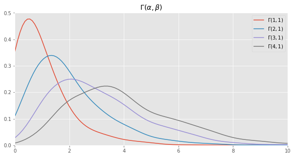
Here we make 1,000 samples from gamma distributions parameterized differently and plot the density curves.
[3]:
fig, ax = plt.subplots(1, 1, figsize=(10, 5))
ax.set_xlim([0, 10])
ax.set_title(r'$\Gamma(\alpha, \beta)$')

_ = sns.kdeplot([rgama(1) for _ in range(1000)], bw=0.5, ax=ax, label=r'$\Gamma(1, 1)$')
_ = sns.kdeplot([rgama(2) for _ in range(1000)], bw=0.5, ax=ax, label=r'$\Gamma(2, 1)$')
_ = sns.kdeplot([rgama(3) for _ in range(1000)], bw=0.5, ax=ax, label=r'$\Gamma(3, 1)$')
_ = sns.kdeplot([rgama(4) for _ in range(1000)], bw=0.5, ax=ax, label=r'$\Gamma(4, 1)$')
3.3. Dirichlet
Here we sample 1 set of probabilities from a Dirichlet distribution with the \(\alpha\)’s as \(\mathrm{\alpha} = [\alpha_1, \alpha_2] = [1, 2]\). We then estimate the (log) probability of these probabilities for two Dirichlet distribution parameterized differently.
[4]:
alphas = np.array([1, 2])
x = rdirch(alphas)

params = [
    np.array([1, 2]),
    np.array([1, 3]),
    np.array([5, 5]),
    np.array([5, 1])
]
print(f'estimating the probability of {x}')

pd.DataFrame([(p, ddirch(x, p)) for p in params], columns=['alphas', 'probability'])
estimating the probability of [0.8011123776705179, 0.198887622329482]
[4]:
| alphas | probability | |
|---|---|---|
| 0 | [1, 2] | -2.654736 |
| 1 | [1, 3] | -3.838228 |
| 2 | [5, 5] | -6.565092 |
| 3 | [5, 1] | -1.221732 |
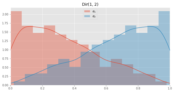
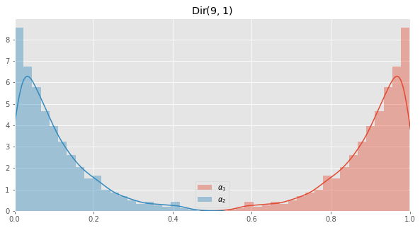
Here we sample data points from two Dirichlet distributions and plot the density of the samples.
\(\operatorname{Dir}(\alpha_1=1, \alpha_2=2)\)
\(\operatorname{Dir}(\alpha_1=9, \alpha_2=1)\)
[5]:
fig, ax = plt.subplots(1, 1, figsize=(10, 5))
ax.set_xlim([0, 1])
ax.set_title(r'$\operatorname{Dir}(1, 2)$')
x = np.array([rdirch(np.array([1, 2])) for _ in range(1000)])
_ = sns.distplot(x[:, 0], ax=ax, label=r'$\alpha_1$')
_ = sns.distplot(x[:, 1], ax=ax, label=r'$\alpha_2$')
_ = plt.legend()

fig, ax = plt.subplots(1, 1, figsize=(10, 5))
ax.set_xlim([0, 1])
ax.set_title(r'$\operatorname{Dir}(9, 1)$')
x = np.array([rdirch(np.array([9, 1])) for _ in range(1000)])
_ = sns.distplot(x[:, 0], ax=ax, label=r'$\alpha_1$')
_ = sns.distplot(x[:, 1], ax=ax, label=r'$\alpha_2$')
_ = plt.legend()
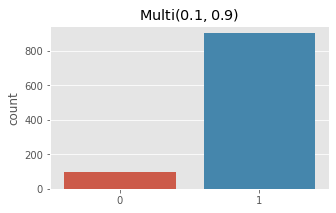
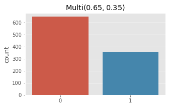
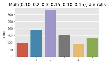
3.4. Multinomial
Here we sample from the Multinomial distribution using different parameters. One of these sampling is for the die example at the beggining.
[6]:
num_ones = 0
for i in range(1000):
    v = rmultnomial(np.array([0.1, 0.9]))
    if v == 1:
        num_ones += 1

print('k = 2, p = [0.1, 0.9]')
print(num_ones / 1000.)

num_zeros = 0
num_ones = 0
num_twos = 0

for i in range(1000):
    v = rmultnomial(np.array([0.1, 0.8, 0.1]))
    if v == 0:
        num_zeros += 1
    elif v == 1:
        num_ones += 1
    else:
        num_twos += 1

print('')
print('k = 3, p = [0.1, 0.8, 0.1]')
print(num_zeros / 1000.)
print(num_ones / 1000.)
print(num_twos / 1000.)

die_counts = np.zeros(6)
for i in range(1000):
    v = rmultnomial(np.array([0.10, 0.2, 0.3, 0.15, 0.10, 0.15]))
    die_counts[v] += 1
sum_counts = np.sum(die_counts)
die_counts = [c / sum_counts for c in die_counts]
print('')
print('k = 6, p = [0.1, 0.2, 0.3, 0.15, 0.10, 0.15], rolling a die')
for i, p in enumerate(die_counts):
    print('{}: {}'.format(i+1, p))
k = 2, p = [0.1, 0.9]
0.895

k = 3, p = [0.1, 0.8, 0.1]
0.106
0.793
0.101

k = 6, p = [0.1, 0.2, 0.3, 0.15, 0.10, 0.15], rolling a die
1: 0.083
2: 0.197
3: 0.31
4: 0.147
5: 0.079
6: 0.184
[7]:
fig, ax = plt.subplots(1, 1, figsize=(5, 3))
ax.set_title(r'$\operatorname{Multi}(0.1, 0.9)$')
x = np.array([rmultnomial(np.array([0.1, 0.9])) for _ in range(1000)])
_ = sns.countplot(x)

fig, ax = plt.subplots(1, 1, figsize=(5, 3))
ax.set_title(r'$\operatorname{Multi}(0.65, 0.35)$')
x = np.array([rmultnomial(np.array([0.65, 0.35])) for _ in range(1000)])
_ = sns.countplot(x)

fig, ax = plt.subplots(1, 1, figsize=(5, 3))
ax.set_title(r'$\operatorname{Multi}(0.10, 0.2, 0.3, 0.15, 0.10, 0.15)$, die rolls')
x = np.array([rmultnomial(np.array([0.10, 0.2, 0.3, 0.15, 0.10, 0.15])) for _ in range(1000)])
_ = sns.countplot(x)
Now we estimate log probability of a sample for Multinomial distributions parameterized differently.
[8]:
import warnings

with warnings.catch_warnings(record=True):
    sample = np.array([2, 8])
    params = [np.array([p, 1.0 - p]) for p in np.linspace(0, 1, 11)]
    sparams = ['[' + ', '.join(['{:.3f}'.format(i) for i in p]) + ']' for p in params]

    df = pd.DataFrame([(s, dmultinomial(sample, p)) for p, s in zip(params, sparams)],
        columns=['parameters', 'probability'])
df
[8]:
| parameters | probability | |
|---|---|---|
| 0 | [0.000, 1.000] | -inf |
| 1 | [0.100, 0.900] | -5.929033 |
| 2 | [0.200, 0.800] | -5.485003 |
| 3 | [0.300, 0.700] | -5.742324 |
| 4 | [0.400, 0.600] | -6.400165 |
| 5 | [0.500, 0.500] | -7.412451 |
| 6 | [0.600, 0.400] | -8.832956 |
| 7 | [0.700, 0.300] | -10.826111 |
| 8 | [0.800, 0.200] | -13.802769 |
| 9 | [0.900, 0.100] | -19.112381 |
| 10 | [1.000, 0.000] | -inf |
3.5. Dirichlet-multinomial
Here’s the last example of sampling from a Dirichlet-Multinomial distribution and then estimating the probality of observed counts using the Dirichlet-Multinomial distributions parameterized differently.
[9]:
count_0 = 0
count_1 = 0

for i in range(100):
    v = rdirmultinom(np.array([2, 8]))
    if v == 0:
        count_0 += 1
    else:
        count_1 += 1

print('estimating probability of count_0 = {}, count_1 = {}'.format(count_0, count_1))

sample = np.array([count_0, count_1])
params = [np.array([alpha_0, 10.0 - alpha_0]) for alpha_0 in np.linspace(0, 10, 11)]

pd.DataFrame([(p, ddirmultinom(sample, p)) for p in params],
             columns=['alphas', 'probability'])
estimating probability of count_0 = 17, count_1 = 83
[9]:
| alphas | probability | |
|---|---|---|
| 0 | [0.0, 10.0] | -0.065782 |
| 1 | [1.0, 9.0] | 0.185436 |
| 2 | [2.0, 8.0] | 0.535957 |
| 3 | [3.0, 7.0] | -0.208196 |
| 4 | [4.0, 6.0] | -0.482921 |
| 5 | [5.0, 5.0] | -0.523687 |
| 6 | [6.0, 4.0] | -0.374440 |
| 7 | [7.0, 3.0] | 0.009409 |
| 8 | [8.0, 2.0] | 0.863991 |
| 9 | [9.0, 1.0] | 0.625902 |
| 10 | [10.0, 0.0] | 0.489876 |
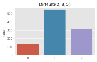
Finally, we sample from a Dirichlet-Multinomial distribution and plot the observed counts.
[10]:
fig, ax = plt.subplots(1, 1, figsize=(5, 3))
ax.set_title(r'$\operatorname{DirMulti}(2, 8, 5)$')
x = np.array([rdirmultinom(np.array([2, 8, 5])) for _ in range(1000)])
_ = sns.countplot(x)
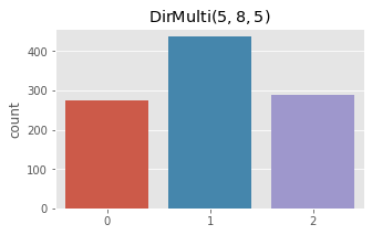
fig, ax = plt.subplots(1, 1, figsize=(5, 3))
ax.set_title(r'$\operatorname{DirMulti}(5, 8, 5)$')
x = np.array([rdirmultinom(np.array([5, 8, 5])) for _ in range(1000)])
_ = sns.countplot(x)
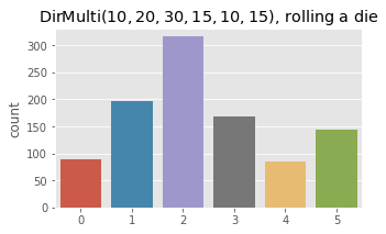
fig, ax = plt.subplots(1, 1, figsize=(5, 3))
ax.set_title(r'$\operatorname{DirMulti}(10, 20, 30, 15, 10, 15)$, rolling a die')
x = np.array([rdirmultinom(np.array([10, 20, 30, 15, 10, 15])) for _ in range(1000)])
_ = sns.countplot(x)